1. Why Machine Learning Feels Different From Traditional Programming
Imagine that you want to build an email spam filter.
In traditional programming, you would sit down and write rules such as:
- If the message contains “win money”, mark it as suspicious.
- If the sender is unknown and the message has many links, raise the risk score.
- If the email contains certain blocked keywords, move it to spam.
That approach works for a while, but spammers adapt quickly. They change wording, hide links, or imitate normal emails. Soon, the rule list becomes large, brittle, and hard to maintain.
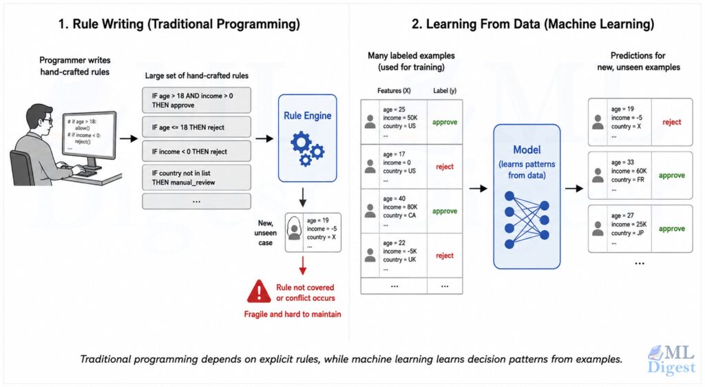
Machine learning changes the approach. Instead of writing every rule by hand, you show the system many examples of spam and non-spam emails. The model learns patterns from data and produces predictions for new messages it has never seen before.
That is the central idea of machine learning: rather than explicitly coding every decision rule, we train a system to learn useful patterns from examples.
2. What Machine Learning Is
Machine learning is a field of computer science and statistics focused on building systems that improve at a task by learning from data.
At a high level, a machine learning system does three things:
- It observes examples.
- It finds patterns that help solve a task.
- It uses those learned patterns to make predictions or decisions on new data.
In short, machine learning is the practice of learning a function that maps inputs to useful outputs.
Examples:
- Input: house details such as size, location, and age. Output: predicted price.
- Input: bank transaction history. Output: fraud probability.
- Input: customer behavior. Output: churn risk.
- Input: product images. Output: predicted category.
Machine Learning is not a new concept. Check the detailed History & Evolution of Machine Learning. Here’s a brief look at its journey:
- 1950s: Groundwork for machine learning by exploring logic, human reasoning, and computation.
- 1956: The Dartmouth Conference, considered the birthplace of AI
- 1960s-2000s: Growth in algorithms and computational power enabled richer model development like neural network, SVM, expert systems, etc.
- 2010s-Present: Explosion of data and advances in deep neural networks lead to breakthroughs in text, image and speech related applications.
3. Why Machine Learning Matters
Machine learning matters because many real-world problems are too messy for pure rule-based programming.
Consider a few common situations:
- It is hard to write exact rules for complex real-world tasks such as recognizing faces, classifying documents, or translating languages.
- Patterns change over time, as seen in fraud detection, recommendation systems, and demand forecasting.
- The signal is distributed across many weak clues rather than one obvious rule.
This is why machine learning appears across modern products and services. If you want a broader survey, see real-world applications of ML. Typical examples include search ranking, recommendation systems, self-driving research, medical imaging, industrial quality inspection, and large language models.
4. Machine Learning, Artificial Intelligence, and Deep Learning
These terms are related, but they are not the same.
- Artificial intelligence is the broad goal of building systems that perform tasks associated with human intelligence.
- Machine learning is a major subset of artificial intelligence that relies on statistical methods to learn from data.
- Deep learning is a specialized subset of machine learning that uses multi-layer artificial neural networks to model complex patterns.
One useful mental model is this:
- AI is the full umbrella.
- ML is a practical method inside AI.
- Deep learning is one powerful family inside ML.
5. The Main Types of Machine Learning
5.1 Supervised Learning
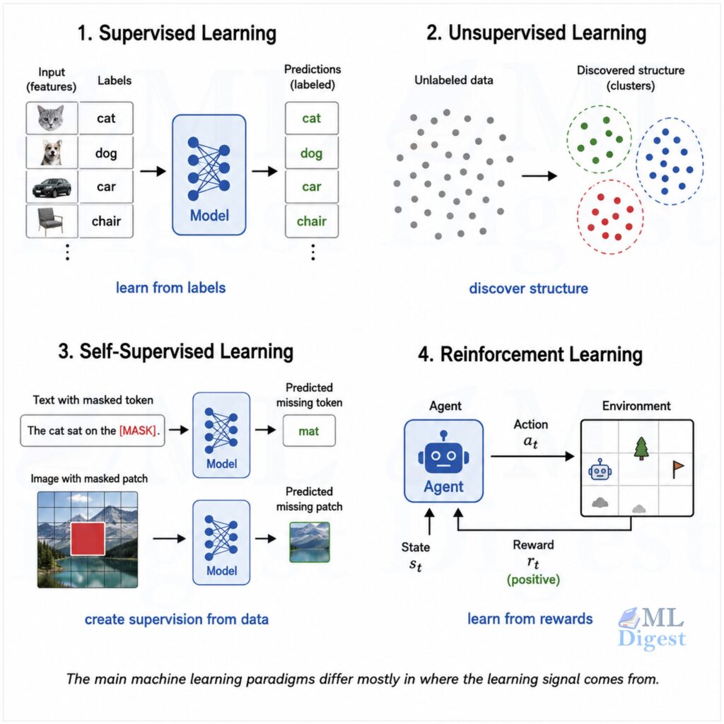
In supervised learning, the model learns from labeled examples. Each training example includes both an input and the correct answer.
Examples:
- Predicting a house price from property features.
- Predicting whether a loan will default.
- Classifying an image as cat, dog, or bird.
Common supervised tasks:
- Regression, where the output is a continuous number.
- Classification, where the output is a category or class.
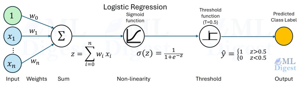
Common algorithms include linear regression, logistic regression, decision trees, random forests, gradient-boosted trees such as XGBoost, and neural networks.
5.2 Unsupervised Learning
In unsupervised learning, the data has no labels. The model tries to discover structure on its own.
Examples:
- Grouping customers into segments.
- Detecting unusual patterns in network traffic.
- Compressing high-dimensional data into a smaller representation.
Common tasks:
- Clustering, where the goal is to group similar data points together.
- Dimensionality reduction, where the goal is to reduce the number of features while preserving important information.
- Anomaly detection, which is often treated as an unsupervised or weakly supervised problem when labeled anomalies are scarce.
Common algorithms include K-means clustering, Gaussian mixture models, principal component analysis (PCA), and autoencoders. If you want a higher-level entry point for this part of the field, see this introduction to ML clustering and this overview of anomaly detection.
5.3 Self-Supervised Learning
Self-supervised learning sits between supervised and unsupervised learning. The model creates supervision signals from the data itself.
For example, in language modeling, a model learns to predict the next token in a sequence. In image learning, a model may learn to reconstruct masked image patches.
This idea powers many modern foundation models, including BERT and GPT-style models.
5.4 Reinforcement Learning
In reinforcement learning, an agent interacts with an environment and learns by trial and error through rewards.
Examples:
- Game playing
- Robot control
- Ad placement and sequential decision-making
The central question becomes: which sequence of actions will maximize long-term reward?
For a non-ML beginner, the key takeaway is that reinforcement learning is usually about sequential decisions, while supervised learning is usually about learning from examples with known answers. For a fuller beginner-oriented walkthrough, see this introduction to reinforcement learning.
6. A Visual Overview of the Machine Learning Workflow
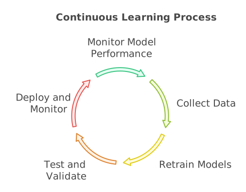
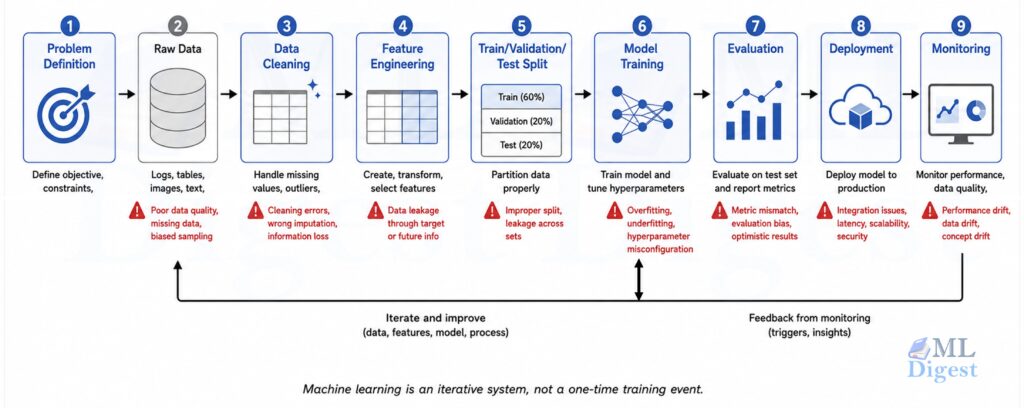
Most machine learning projects follow a loop rather than a straight line. The main stages can be seen from the diagram below. For the end-to-end version beyond this primer, see the machine learning project lifecycle guide.
7. The Core Building Blocks You Need to Understand
7.1 Data, Features, Labels, and Targets
Every machine learning task starts with data. You can think of a dataset as a table:
- Rows are examples.
- Columns are features.
- One special column may be the target or label.
Example for house-price prediction:
- Features: square footage, number of bedrooms, location, age of property.
- Target: sale price.
Example for email classification:
- Features: message length, number of links, word frequencies, sender reputation.
- Target: spam or not spam.
In notation, we often write:
$$
X \in \mathbb{R}^{n \times d}, \quad y \in \mathbb{R}^{n}
$$
where $n$ is the number of examples, $d$ is the number of features, $X$ is the input feature matrix, and $y$ is the target vector.
7.2 The Model
A model is a mathematical function that maps inputs to outputs.
We often write:
$$
\hat{y} = f(x; \theta)
$$
where $x$ is an input example, $\theta$ represents the model parameters, and $\hat{y}$ is the predicted output.
For a linear regression model, that function might look like this:
$$
\hat{y} = w^T x + b
$$
This means the prediction is a weighted combination of input features plus a bias term.
Even very complex models, including deep neural networks, still follow the same basic idea: input goes in, parameters transform it, and a prediction comes out.
7.3 The Loss Function
The model needs a way to measure how wrong it is. That measurement is called the loss function.
For regression, a common choice is mean squared error (MSE):
$$
\operatorname{MSE} = \frac{1}{n} \sum_{i=1}^{n} (y_i – \hat{y}_i)^2
$$
This penalizes large errors more strongly because the difference is squared.
For binary classification, a common choice is cross-entropy loss:
$$
\mathcal{L} = -\frac{1}{n} \sum_{i=1}^{n} \left[y_i \log(\hat{p}_i) + (1-y_i) \log(1-\hat{p}_i)\right]
$$
Here, $\hat{p}_i$ is the predicted probability that example $i$ belongs to the positive class.
The role of training is simple to state: find parameter values that make the loss small on useful data.
7.4 Optimization and Gradient Descent
Once we define a model and a loss function, we need a way to improve the parameters.
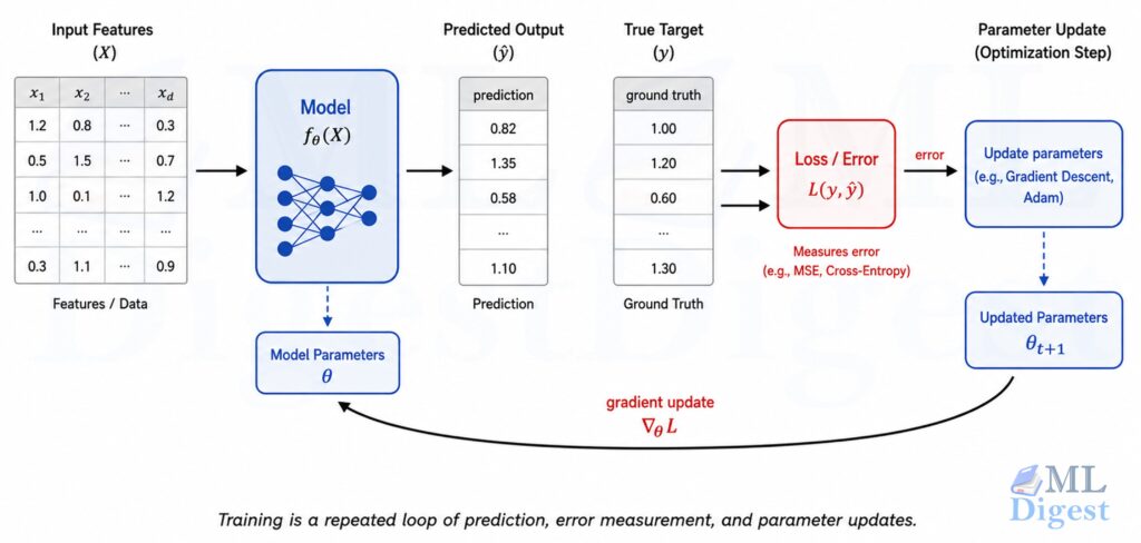
One standard method is gradient descent. At each step, we compute how the loss changes with respect to the parameters and move the parameters in the direction that reduces the loss.
The update rule is:
$$
w \leftarrow w – \eta \nabla_w \mathcal{L}
$$
where $w$ are the parameters, $\eta$ is the learning rate, and $\nabla_w \mathcal{L}$ is the gradient of the loss with respect to the parameters.
Intuitively, this is like walking downhill on a landscape where height represents error. The gradient tells you which direction points uphill, so you step the other way.
7.5 Training, Validation, and Test Data
One of the most important ideas in machine learning is generalization. A model is useful only if it performs well on new data, not only on the examples it already saw during training.
This is why datasets are usually split into three parts:
- Training set: used to fit model parameters.
- Validation set: used to tune choices such as model type, hyperparameters, or preprocessing steps.
- Test set: used once at the end for a final, unbiased estimate.
If you tune decisions based on the test set again and again, the test set stops being a fair test.
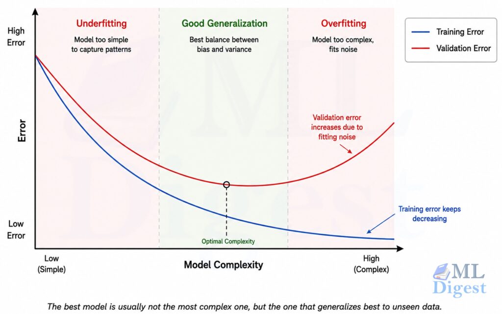
7.6 Overfitting and Underfitting
Underfitting happens when a model is too simple to capture the pattern.
Overfitting happens when a model fits the training data too closely, including noise, and then performs poorly on new data.
This tradeoff is central to machine learning and is usually discussed as the bias-variance tradeoff.
Signs of underfitting:
- Poor training performance
- Poor validation performance
Signs of overfitting:
- Very strong training performance
- Noticeably worse validation or test performance
Common ways to reduce overfitting:
- Collect more representative data
- Use simpler models or stronger regularization
- Reduce data leakage
- Use cross-validation when appropriate
- Stop training earlier in neural networks
8. How Models Are Evaluated
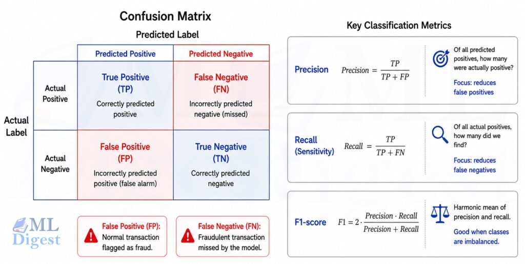
Different tasks need different metrics.
For regression mean squared error (MSE), mean absolute error (MAE), and $R^2$ are common choices.
For classification accuracy, precision, recall, F1-score, and ROC-AUC are common choices.
Accuracy alone can be misleading. For example, if 99 percent of transactions are normal, a model that always predicts “normal” has 99 percent accuracy and still fails at fraud detection.
That is why evaluation must match the business problem.
Examples:
- In medical screening, high recall may matter because missing a true case is costly.
- In spam filtering, you may care about both precision and recall because you do not want to block important emails.
- In recommendation systems, ranking metrics often matter more than raw accuracy.
9. Common Model Families and When People Use Them
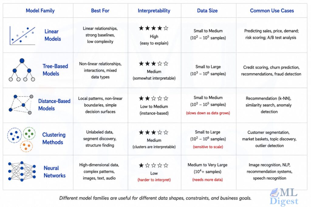
9.1 Linear Models
Linear regression and logistic regression are often the right starting point. They are fast, interpretable, and strong baselines on many small structured datasets.
Use them when:
- You want a strong baseline quickly.
- Interpretability matters.
- The relationship is reasonably simple or can be approximated well.
9.2 Tree-Based Models
Decision trees, random forests, XGBoost, LightGBM, and CatBoost are strong choices for tabular business data.
Use them when:
- You have mixed structured features, often with categorical columns that may need encoding depending on the library.
- Feature interactions matter.
- You want high performance without building a deep neural network.
In practice, boosted trees are often a very strong baseline on structured data.
9.3 Distance-Based Models
Algorithms such as k-nearest neighbors rely on similarity between examples.
Use them when:
- The dataset is small enough to compare examples directly.
- Local similarity is meaningful.
9.4 Clustering and Representation Learning
If the goal is to discover hidden structure rather than predict a label, clustering or dimensionality reduction methods are common.
Use them when:
- You want customer segments.
- You want to visualize high-dimensional data.
- You need data exploration before building a supervised model.
9.5 Neural Networks and Deep Learning
Neural networks are especially useful when the input is complex and unstructured, such as text, images, audio, or video.
Use them when:
- You have large datasets.
- The problem involves highly complex patterns.
- You are working on computer vision, speech, or natural language processing.
Frameworks such as PyTorch and TensorFlow are commonly used for these systems.
9.6 Where Large Language Models Fit In
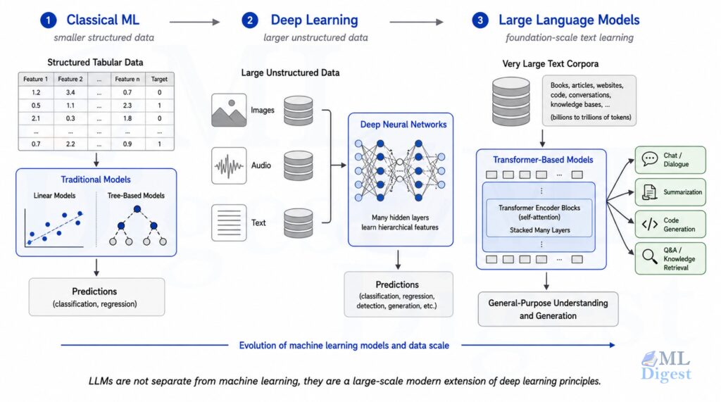
Large language models (LLMs) are machine learning models trained on large text corpora, usually using deep learning and self-supervised learning objectives. If you want to see how this family evolved from earlier neural language models into modern systems, see this overview of LLM architecture evolution.
So when people ask whether LLMs are part of machine learning, the answer is yes. They are a modern and highly visible branch of machine learning, not a separate universe.
What makes them special is scale:
- Very large neural networks
- Very large datasets
- Significant compute during training
- Strong general-purpose behavior across many downstream tasks
The core ideas are still recognizable: data, parameters, loss function, optimization, evaluation, and deployment. The difference is that LLMs operate at a scale that was not common in earlier machine learning systems.
10. A Small but Real Machine Learning Example in Python
The code below trains a simple classifier on the Iris dataset using scikit-learn. The goal is to predict the flower species from basic measurements.
This is not a glamorous production example, but it shows the complete beginner workflow:
- Load data.
- Split into train and test sets.
- Build a preprocessing and modeling pipeline.
- Train the model.
- Evaluate on unseen data.
from sklearn.datasets import load_iris
from sklearn.linear_model import LogisticRegression
from sklearn.metrics import accuracy_score, classification_report, confusion_matrix
from sklearn.model_selection import train_test_split
from sklearn.pipeline import make_pipeline
from sklearn.preprocessing import StandardScaler

# 1. Load a small built-in dataset.
iris = load_iris()
X = iris.data
y = iris.target

# 2. Create train and test splits.
X_train, X_test, y_train, y_test = train_test_split(
    X,
    y,
    test_size=0.2,
    random_state=42,
    stratify=y,
)

# 3. Build a simple pipeline.
#    StandardScaler normalizes the input features.
#    LogisticRegression learns a linear decision boundary.
model = make_pipeline(
    StandardScaler(),
    LogisticRegression(max_iter=1000)
)

# 4. Train the model.
model.fit(X_train, y_train)

# 5. Run predictions on unseen test data.
y_pred = model.predict(X_test)

# 6. Evaluate the model.
print("Accuracy:", accuracy_score(y_test, y_pred))
print("\nClassification report:\n")
print(classification_report(y_test, y_pred, target_names=iris.target_names))
print("Confusion matrix:\n", confusion_matrix(y_test, y_pred))What this example teaches:
- Data is split before evaluation.
- Preprocessing is part of the pipeline.
- The model is trained on one subset and tested on another.
- The final number is not magic, it is the result of careful data handling and evaluation.
If you run this example, you will usually get strong performance because the Iris dataset is small and clean. Real production datasets are much messier.
11. Tools and Technologies for Machine Learning
Once beginners understand the basic workflow, the next practical question is: what tools do people actually use?
The answer depends on the type of work. Some tools are best for quick experimentation, some are better for production systems, and some help with deployment and monitoring.
11.1 Programming Languages
Python is the dominant language in machine learning because it has the strongest ecosystem of libraries, tutorials, and community support.
It is widely used for data analysis, model training, experimentation, deep learning research, and production inference services.
Other languages also appear in practice:
- R is common in statistics-heavy workflows and academic analysis.
- SQL is essential for querying, joining, and validating data.
- Java, C++, Rust, and Go may be used in production systems where latency, integration, or systems control matters.
For beginners, Python plus basic SQL is usually the most useful starting point.
11.2 Data Handling and Analysis Tools
Before training a model, teams usually spend significant time exploring and cleaning data.
Common tools include:
- NumPy for numerical arrays and mathematical operations.
- pandas for tabular data manipulation.
- Matplotlib and Seaborn for visualization.
- Jupyter notebooks for interactive experimentation.
These tools are often where real ML work begins, because bad data handling can ruin a project before modeling even starts.
11.3 Machine Learning Libraries
Different libraries are useful for different problem types.
- scikit-learn is the standard starting point for classical machine learning. It is excellent for linear models, trees, clustering, preprocessing, and evaluation.
- XGBoost, LightGBM, and CatBoost are widely used for high-performance tabular modeling.
- PyTorch and TensorFlow are the main deep learning frameworks for neural networks.
- Hugging Face Transformers is commonly used for modern NLP and many foundation-model workflows.
As a practical rule:
- Use scikit-learn for beginner projects and structured data baselines.
- Use boosted-tree libraries for strong tabular-data performance.
- Use PyTorch or TensorFlow when working with deep learning.
11.4 Data Storage and Processing Technologies
Machine learning rarely happens in isolation from data infrastructure.
Teams often rely on:
- Relational databases such as PostgreSQL or MySQL
- Data warehouses such as BigQuery, Snowflake, or Redshift
- Distributed processing tools such as Apache Spark
- Object storage such as Amazon S3, Azure Blob Storage, or Google Cloud Storage
The core idea is simple: models depend on reliable access to good data, and that usually requires more than a single CSV file on a laptop.
11.5 Experiment Tracking and Reproducibility Tools
As projects become more serious, teams need to keep track of datasets, model versions, hyperparameters, and results.
Common tools include:
- MLflow for experiment tracking and model management.
- Weights & Biases for experiment logging and visualization.
- DVC for dataset and pipeline versioning.
- Git for code version control.
Without this layer, it becomes hard to answer basic questions such as: Which dataset produced this model? Which hyperparameters were used? Why did last week’s version perform better? For a concrete tool in this space, see this MLflow guide.
11.6 Deployment and Serving Technologies
Training a model is only part of the job. A useful model usually needs to be served to real users or business systems.
Common deployment patterns include:
- Batch prediction jobs for scheduled scoring.
- Real-time APIs using tools such as FastAPI or Flask.
- Containerized deployment with Docker and Kubernetes.
- Cloud ML platforms such as AWS SageMaker, Azure Machine Learning, and Google Vertex AI.
For smaller projects, a simple Python API may be enough. For larger systems, deployment usually becomes a broader software engineering problem.
11.7 Monitoring and Operations
Once a model is live, teams need to monitor both technical behavior and business impact.
This may include:
- Input data drift
- Prediction drift
- Latency and error rates
- Resource usage
- Business metrics tied to model outcomes
Common operational tools may include logging systems, dashboards, alerting platforms, and specialized ML monitoring products.
The important beginner lesson is that machine learning is not only about training models. It also depends on data tools, software infrastructure, deployment systems, and monitoring practices.
12. What Usually Makes Machine Learning Projects Fail
Beginners often assume the hardest part is choosing a fancy model. In real projects, failure usually comes from more basic issues.
12.1 Poor Problem Framing
If the target is vague, the model will not help.
Bad framing: “Predict customer success”
Better framing: “Predict whether a customer will cancel their subscription in the next 30 days”
The second version is measurable and time-bound.
12.2 Low-Quality or Biased Data
Machine learning inherits the strengths and weaknesses of its data.
Common issues:
- Missing values
- Inconsistent labels
- Sampling bias
- Outdated data
- Data that does not reflect real deployment conditions
If the data is wrong, the model will often be confidently wrong. That is also why handling imbalanced data and ethics and fairness in machine learning are not side topics; they directly affect whether a model is useful and trustworthy.
12.3 Data Leakage
Data leakage happens when information from the future or from the evaluation set accidentally leaks into training. Examples:
- Computing preprocessing statistics on the full dataset before splitting.
- Using a feature that is only known after the prediction target occurs.
- Reusing the test set for repeated tuning.
Leakage can make a weak model look excellent during experimentation and fail immediately in production. A closely related production concern is point-in-time correctness, where features must reflect only what was actually known at prediction time.
12.4 Ignoring the Deployment Environment
A model trained offline may break in production if the live input data looks different. This is often called distribution shift or data drift.
Examples:
- Customer behavior changes over time.
- Sensor hardware changes.
- Input formats evolve.
- The business process itself changes.
13. Best Practices for Non-ML Teams Getting Started
If you are new to machine learning, the safest path is usually the simplest one.
- Start With a Baseline:
Build the simplest reasonable model first. Examples: - Mean prediction for regression
- Majority-class prediction for classification
- Logistic regression or a small tree-based model as the first real baseline
If a complex model does not clearly beat a baseline, it does not deserve the added complexity.
- Improve Data Before Chasing Model Complexity:
Many teams get larger gains from better data labeling, cleaner features, and clearer evaluation than from switching to a more advanced model. - Match the Metric to the Business Cost:
Do not optimize the wrong number. If false negatives are expensive, recall may matter more than accuracy. If ranking matters, use ranking metrics. - Keep the Pipeline Reproducible:
Use fixed random seeds where possible. Save preprocessing choices. Version datasets and models. Make it possible to rerun training and get comparable results. - Separate Experimentation From Final Evaluation:
Use validation data for iteration. Keep a clean test set for the end. - Monitor After Deployment:
Deployment is the beginning of the next phase, not the end of the project.
Monitor the input drift, prediction distributions, latency, failures, and business outcomes. Be ready to retrain or adjust the model as conditions change.
A Practical Learning Path for Beginners
If you want to move from zero familiarity to useful working knowledge, a sensible order is:
- Learn the supervised learning workflow.
- Practice with small structured datasets in scikit-learn.
- Understand train, validation, and test splits.
- Learn metrics, overfitting, and feature preprocessing.
- Study tree-based models and simple linear models.
- Then move into neural networks and deep learning.
Good beginner-friendly resources include:
- scikit-learn user guide
- PyTorch tutorials
- The Elements of Statistical Learning
- Pattern Recognition and Machine Learning
- Machine Learning Yearning
Closing Thoughts
Machine learning is neither magic nor only for specialists. It is a practical toolkit for problems where patterns can be learned from data better than they can be hard-coded by hand.
Machine learning is a disciplined way to use data to learn patterns that generalize to new examples.
The workflow sounds simple, but doing it well requires care in problem definition, data collection, evaluation, and deployment.
For non-ML readers, the most important shift is this:
- Traditional programming says, “write the rules.”
- Machine learning says, “show examples, define the objective, and learn the rules from data.”
You do not need to start with deep learning, advanced math, or large-scale infrastructure. A strong grasp of the basic workflow, a simple model, and a careful evaluation process will take you much farther than most beginners expect.
That is the right foundation. Once you have that, topics such as deep learning, transformers, recommendation systems, and LLMs become extensions of a framework you already understand.

Silpa brings 5 years of experience in working on diverse ML projects, specializing in designing end-to-end ML systems tailored for real-time applications. Her background in statistics (Bachelor of Technology) provides a strong foundation for her work in the field. Silpa is also the driving force behind the development of the content you find on this site.

Happy is a seasoned ML professional with over 15 years of experience. His expertise spans various domains, including Computer Vision, Natural Language Processing (NLP), and Time Series analysis. He holds a PhD in Machine Learning from IIT Kharagpur and has furthered his research with postdoctoral experience at INRIA-Sophia Antipolis, France. Happy has a proven track record of delivering impactful ML solutions to clients.
Subscribe to our newsletter!