Imagine you are a real estate agent. A client walks in and asks: “How much should I list my house for?” You do not flip to a random page in a notebook. Instead, you instinctively recall dozens of homes you have sold, noting their sizes, neighborhoods, number of bedrooms, and the prices they fetched. You draw on that accumulated experience to make a confident estimate. You are, in effect, fitting a mental model that maps measurable features to a predicted price.
Linear regression is exactly this idea, made precise and computational. It is one of the oldest, most interpretable, and most practically useful tools in the entire machine learning toolkit. Do not let its simplicity fool you: the intuitions and mathematics behind linear regression underpin practically every advanced model you will ever build, from neural networks to Gaussian processes.
This guide walks you through linear regression from first principles, covering the intuition, the math, the code, the assumptions, and the practical pitfalls.
By the end, you should be able to answer four questions clearly: what the model is actually learning, why the least-squares objective makes sense, when the method is trustworthy, and what to try when its assumptions begin to fail.
1. The Intuition: A Line That “Fits” the Data
1.1 The Core Idea
Suppose you collect data on 100 apartments: each apartment has one feature (its size in square meters) and one label (its rent in dollars per month). You plot these 100 points on a scatter plot (size on the x-axis, rent on the y-axis).
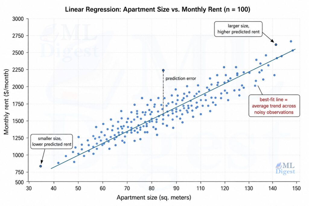
The goal of linear regression is to find the straight line that best summarizes the relationship between size and rent. “Best” means: the line that, when used to predict rent from size, makes the smallest total prediction error across all 100 apartments.
Once you have that line, predicting rent for a new apartment is easy: find its size on the x-axis, trace up to the red line, and read off the y-value. That is your prediction.
1.2 From One Feature to Many
The real power shows up when you have many features at once: size, number of bedrooms, floor level, distance to the nearest metro station. You can no longer draw a simple 2D line. Instead, you fit a hyperplane in a higher-dimensional space. The math is the same (it is still called linear regression), and the intuition is the same: find the flat surface that best fits the scattered cloud of data points.
2. The Mathematical Setup
2.1 Notation
Let us formalize the setting. You have:
- $n$ training examples
- $d$ input features per example
- A feature matrix $\mathbf{X} \in \mathbb{R}^{n \times d}$ where row $i$ is the feature vector $\mathbf{x}^{(i)}$
- A target vector $\mathbf{y} \in \mathbb{R}^n$ where $y^{(i)}$ is the true label for example $i$
We typically prepend a column of 1s to $\mathbf{X}$ to absorb the bias term, making $\mathbf{X} \in \mathbb{R}^{n \times (d+1)}$.
2.2 The Hypothesis Function
The linear regression model makes predictions as:
$$\hat{y}^{(i)} = \mathbf{w}^\top \mathbf{x}^{(i)} = w_0 + w_1 x_1^{(i)} + w_2 x_2^{(i)} + \cdots + w_d x_d^{(i)}$$
where $\mathbf{w} \in \mathbb{R}^{d+1}$ is the weight vector (also called the parameter vector or coefficient vector). In matrix form for all $n$ examples at once:
$$\hat{\mathbf{y}} = \mathbf{X}\mathbf{w}$$
The phrase linear regression can be slightly misleading at first. “Linear” does not mean the raw input features must appear only as plain, untransformed variables. It means the model is linear in the parameters. If you replace $x$ with features like $x^2$, $\log x$, or interaction terms such as $x_1 x_2$, the model is still linear regression as long as the prediction is a weighted sum of those features.
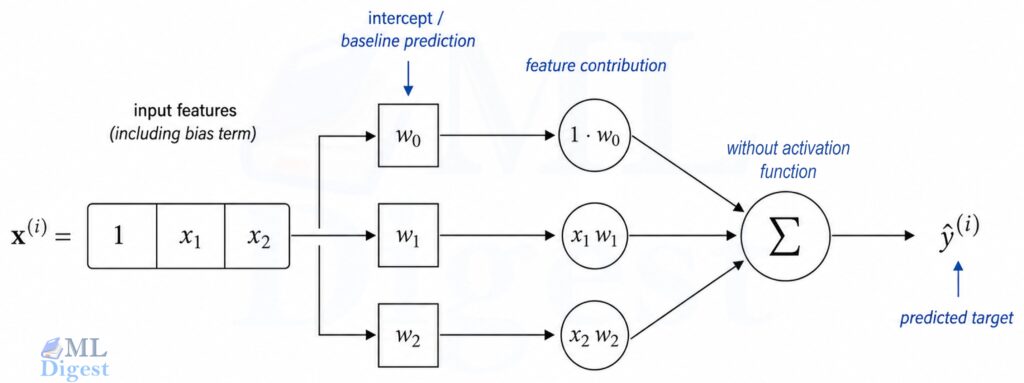
A key connection: A single neuron in a neural network without an activation function is linear regression. Every deep learning model you will ever study is built on exactly this atomic unit.
3. Learning the Parameters: How the Line is Found
3.1 The Cost Function
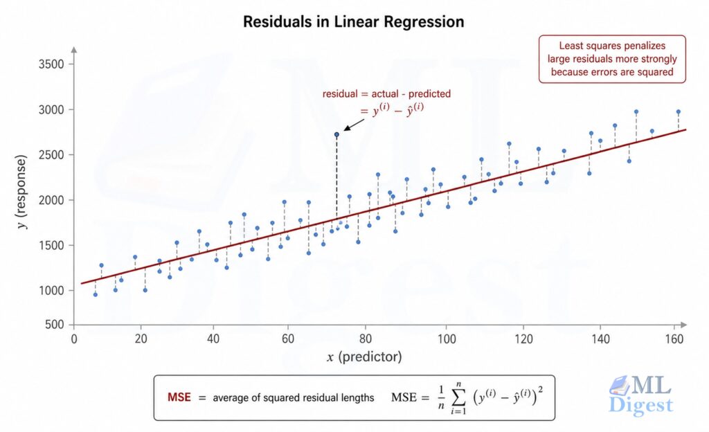
To find the best $\mathbf{w}$, we need to define what “best” means. The standard choice is the Mean Squared Error (MSE):
$$\mathcal{L}(\mathbf{w}) = \frac{1}{n} \sum_{i=1}^{n} \left( y^{(i)} – \hat{y}^{(i)} \right)^2 = \frac{1}{n} | \mathbf{y} – \mathbf{X}\mathbf{w} |^2$$
Why squared error? Three reasons:
- It is differentiable everywhere, so gradient-based optimization works cleanly.
- Large errors are penalized disproportionately more than small ones, so the optimizer naturally focuses on reducing the biggest mistakes first.
- Under the assumption of Gaussian noise, minimizing MSE is equivalent to maximum likelihood estimation (MLE), providing a deep probabilistic justification rather than just a convenient heuristic.
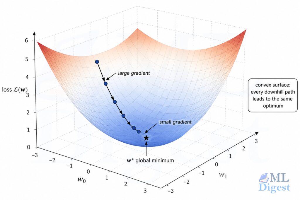
3.2 The Geometry of the Loss Surface
The MSE loss as a function of $\mathbf{w}$ is a convex bowl (more precisely, a quadratic surface). This is an enormously useful property: a convex function has no spurious local minima to get trapped in. If the columns of $\mathbf{X}$ are linearly independent, the minimum is unique. If they are not, multiple parameter vectors can achieve the same minimum training loss, which is one reason regularization becomes helpful.
3.3 The Normal Equation: Solving it Analytically
Because the loss is a smooth convex function, you can find $\mathbf{w}^*$ by setting the gradient to zero and solving algebraically:
$$\nabla_\mathbf{w} \mathcal{L}(\mathbf{w}) = -\frac{2}{n} \mathbf{X}^\top (\mathbf{y} – \mathbf{X}\mathbf{w}) = \mathbf{0}$$
Rearranging:
$$\mathbf{X}^\top \mathbf{X} \mathbf{w} = \mathbf{X}^\top \mathbf{y}$$
$$\boxed{\mathbf{w}^* = (\mathbf{X}^\top \mathbf{X})^{-1} \mathbf{X}^\top \mathbf{y}}$$
This is the Normal Equation, a closed-form exact solution. No iterations, no learning rate to tune.
Strictly speaking, this boxed form requires $\mathbf{X}^\top \mathbf{X}$ to be invertible. When it is singular or nearly singular, the more robust practical statement is that least squares is solved with the Moore-Penrose pseudoinverse:
$$\mathbf{w}^* = \mathbf{X}^+ \mathbf{y}$$
When is the Normal Equation practical?
- It requires inverting the $d \times d$ matrix $\mathbf{X}^\top \mathbf{X}$, an $O(d^3)$ operation.
- For small to medium feature counts (up to around $d \sim 10{,}000$ features), this is fast. For $d = 100{,}000$ features, it becomes computationally infeasible.
- If $\mathbf{X}^\top \mathbf{X}$ is singular (i.e., features are linearly dependent / perfect multicollinearity exists), the inverse does not exist. In practice, the pseudoinverse or regularization handles this.
3.4 Gradient Descent: Solving it Iteratively
When the dataset is too large for the Normal Equation, gradient descent is the standard alternative. The update rule is:
$$\mathbf{w} \leftarrow \mathbf{w} – \alpha \nabla_\mathbf{w} \mathcal{L}(\mathbf{w}) = \mathbf{w} – \frac{2\alpha}{n} \mathbf{X}^\top (\mathbf{X}\mathbf{w} – \mathbf{y})$$
where $\alpha$ is the learning rate, a hyperparameter controlling the step size toward the minimum.
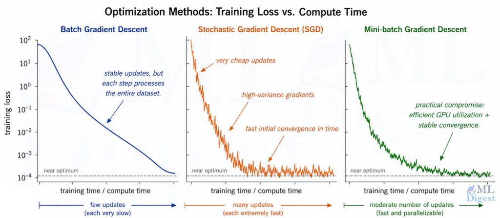
There are three variants:
| Variant | Data used per update | Characteristics |
|---|---|---|
| Batch GD | Full dataset | Stable convergence; slow per step for large $n$ |
| Stochastic GD (SGD) | 1 example | Fast per step; noisy gradient estimates |
| Mini-batch GD | $b$ examples (e.g., 32 or 256) | Best of both worlds; the standard in practice |
These same update rules reappear when training neural networks; Optimization Techniques in Neural Networks covers momentum, Adam, and other variants built on this foundation.
4. Probabilistic Interpretation
It is worth pausing to ask: why MSE specifically? The answer connects linear regression to the rich theory of probabilistic models.
Assume the true relationship is:
$$y^{(i)} = \mathbf{w}^\top \mathbf{x}^{(i)} + \epsilon^{(i)}, \quad \epsilon^{(i)} \sim \mathcal{N}(0, \sigma^2)$$
In other words, the target is the linear prediction plus Gaussian noise. Under this model, the likelihood of the data given $\mathbf{w}$ is:
$$p(\mathbf{y} \mid \mathbf{X}, \mathbf{w}) = \prod_{i=1}^{n} \mathcal{N}(y^{(i)}; \mathbf{w}^\top \mathbf{x}^{(i)}, \sigma^2)$$
In plain English, this formula asks: “How likely is it that our model produced the data we actually observed?” Breaking it down piece by piece:
- $p(\mathbf{y} \mid \mathbf{X}, \mathbf{w})$ : the probability of seeing our observed targets, given the features and our current weights.
- $\mathcal{N}(y^{(i)}; \mathbf{w}^\top \mathbf{x}^{(i)}, \sigma^2)$ : for each data point, this asks: “how probable is this actual value, if the model predicted $\mathbf{w}^\top \mathbf{x}^{(i)}$ with some noise?” Think of it like a dart thrower who always aims at the bullseye but lands slightly off. Points close to the prediction get high probability; points far away get low probability.
- $\prod_{i=1}^{n}$ : we multiply across all $n$ examples, because we assume each one is independent (like multiplying the probabilities of independent coin flips).
Good weights make predictions close to the true values, so each $\mathcal{N}(\cdots)$ term is large, and the whole product is large. Finding $\mathbf{w}$ that maximizes this probability is MLE.
Taking the log-likelihood and maximizing with respect to $\mathbf{w}$ yields exactly the same objective as minimizing MSE. Minimizing MSE = Maximum Likelihood Estimation under Gaussian noise. This is not a coincidence. It is the reason we use MSE for regression in the first place.
This probabilistic framing connects to a classical optimality result. Under the assumptions described in Section 5, the Gauss-Markov theorem guarantees that OLS is the Best Linear Unbiased Estimator (BLUE): among all linear unbiased estimators, OLS achieves the smallest variance for each coefficient. This guarantee requires only that the noise has zero mean and constant finite variance; the Gaussian assumption is not needed for BLUE, but it is needed for the MLE equivalence above.
5. The Assumptions of Linear Regression
Every model comes with assumptions. Violating them does not always break the model, but it helps to know why things go wrong when they do. It is also useful to separate two goals:
- If your goal is prediction, mild assumption violations may still leave you with a useful model.
- If your goal is interpreting coefficients, estimating uncertainty, or making causal claims, the assumptions matter much more.
The classical assumptions are often summarized in simplified acronyms such as LINE, but in practice it is better to think through each requirement explicitly:
5.1 Linearity
The relationship between features and the target must be linear (in the parameters). If the true relationship is curved, the linear model will systematically underfit.
Diagnostic: Plot residuals vs. fitted values. A curved or systematic pattern signals non-linearity.
Fix: Add polynomial features (e.g., $x_1^2$, $x_2^3$, $x_1x_2$), apply a log transform to skewed variables, or switch to a non-linear model.
5.2 Independence
The residuals must be independent of each other. This is commonly violated in time-series data, where consecutive data points are correlated.
Diagnostic: The Durbin-Watson test or plotting residuals vs. time index (look for autocorrelation patterns).
Fix: Use time-series models (ARIMA, etc.) or add lag features.
5.3 Normality of Residuals
The residuals should be approximately normally distributed (for inference and confidence intervals to be valid). For prediction purposes only, this assumption matters less.
Diagnostic: A Q-Q plot of residuals, or a Shapiro-Wilk normality test.
Fix: Apply a Box-Cox transformation to the target variable.
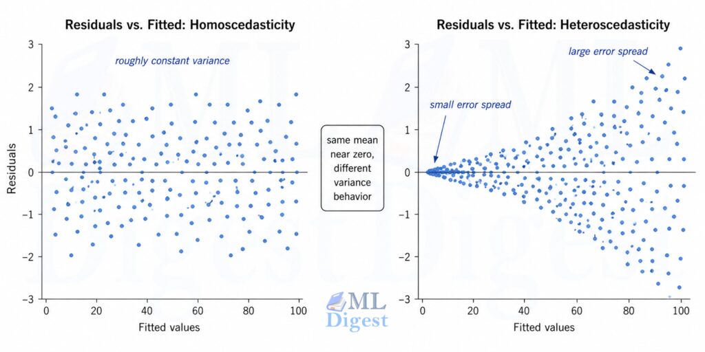
5.4 Equal Variance (Homoscedasticity)
The variance of the residuals should be constant across all levels of the fitted values. If larger predictions tend to have larger errors, you have heteroscedasticity.
Diagnostic: Plot residuals vs. fitted values. A funnel shape signals heteroscedasticity.
Fix: Use Weighted Least Squares (WLS), apply a log transformation to the target, or use robust standard errors.
5.5 No Perfect Multicollinearity
No feature should be an exact linear combination of the others. If one column in $\mathbf{X}$ can be reconstructed perfectly from the rest, the model cannot uniquely determine how much credit to assign to each correlated feature.
Diagnostic: Check the correlation matrix, compute VIF scores, or watch for singular-matrix warnings during fitting.
Fix: Remove one of the redundant features, combine them, or use Ridge regression to stabilize the fit. For a focused exploration of why correlated features destabilize coefficients, see Multicollinearity in Linear Regression.
5.6 Zero Conditional Mean
The error term should have mean zero once the features are known: $\mathbb{E}[\epsilon \mid \mathbf{X}] = 0$. Intuitively, this means the residual should not still contain a systematic pattern that your chosen features failed to capture.
This assumption is easy to overlook, but it is the one that most directly affects coefficient interpretation. If an important variable is omitted and is correlated with an included feature, the coefficient on the included feature becomes biased. This is the classic omitted-variable bias problem.
Diagnostic: Residual plots, domain knowledge, and ablation checks with alternative feature sets are often more informative than any single formal test.
Fix: Add the missing explanatory variables when possible, rethink the feature set, or be explicit that the model is predictive rather than causal.
6. Regularization: When the Line
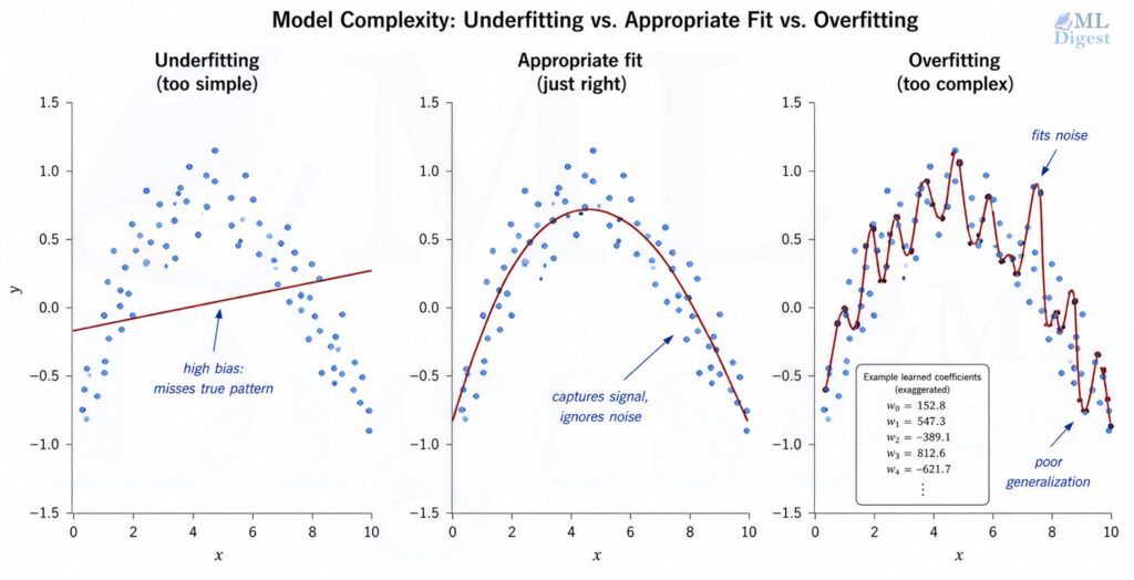
6.1 The Overfitting Problem
When you have more features than you have data, or when features are highly correlated, the least-squares solution can fit the training data very closely while generalizing poorly to new data. The weights become large and erratic, reflecting noise rather than signal. This is overfitting, the central challenge captured by the bias-variance tradeoff.
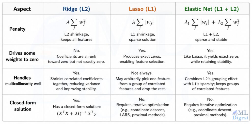
6.2 Ridge Regression (L2 Regularization)
Ridge regression adds a penalty on the squared magnitude of the weights to the loss function:
$$\mathcal{L}_{\text{Ridge}}(\mathbf{w}) = \frac{1}{n}|\mathbf{y} – \mathbf{X}\mathbf{w}|^2 + \lambda |\mathbf{w}|^2$$
The hyperparameter $\lambda \geq 0$ controls the strength of the penalty. The closed-form solution becomes:
$$\mathbf{w}^*_{\text{Ridge}} = (\mathbf{X}^\top \mathbf{X} + \lambda \mathbf{I})^{-1} \mathbf{X}^\top \mathbf{y}$$
Adding $\lambda \mathbf{I}$ to $\mathbf{X}^\top \mathbf{X}$ makes the matrix invertible even in degenerate cases, a practical bonus beyond just regularizing. Ridge shrinks all weights toward zero but never sets them exactly to zero.
Ridge regression also has an elegant Bayesian interpretation: it is equivalent to maximum a posteriori (MAP) estimation when a zero-mean Gaussian prior is placed on the weights. The regularization strength $\lambda$ corresponds to the precision of that prior, and a larger $\lambda$ imposes a tighter prior, pulling the weights more strongly toward zero. This connection generalises naturally: Lasso corresponds to a Laplace (double-exponential) prior, which produces the characteristic sparsity.
6.3 Lasso Regression (L1 Regularization)
Lasso (Least Absolute Shrinkage and Selection Operator) uses the absolute value of the weights as the penalty:
$$\mathcal{L}_{\text{Lasso}}(\mathbf{w}) = \frac{1}{n}|\mathbf{y} – \mathbf{X}\mathbf{w}|^2 + \lambda |\mathbf{w}|_1$$
Unlike Ridge, Lasso drives many weights to exactly zero. This makes Lasso a built-in feature selection mechanism; the non-zero weights after fitting tell you which features actually matter. There is no closed-form solution for Lasso; it requires iterative solvers (e.g., coordinate descent).
6.4 Elastic Net
Elastic Net combines both penalties:
$$\mathcal{L}_{\text{EN}}(\mathbf{w}) = \frac{1}{n}|\mathbf{y} – \mathbf{X}\mathbf{w}|^2 + \lambda_1 |\mathbf{w}|_1 + \lambda_2 |\mathbf{w}|^2$$
It inherits Lasso’s sparsity and Ridge’s stability under multicollinearity. When you are not sure which to use, Elastic Net is a safe default.
7. Evaluation Metrics
After fitting a model, how do you know if it is good? The following metrics are standard:
Mean Absolute Error (MAE):
$$\text{MAE} = \frac{1}{n} \sum_{i=1}^{n} |y^{(i)} – \hat{y}^{(i)}|$$
Interpretable in the same units as the target. Robust to outliers. “On average, my predictions are off by $X$ dollars.”
Root Mean Squared Error (RMSE):
$$\text{RMSE} = \sqrt{\frac{1}{n} \sum_{i=1}^{n} (y^{(i)} – \hat{y}^{(i)})^2}$$
Also in the same units as the target, but penalizes large errors more heavily than MAE. Sensitive to outliers. Preferred when large errors are particularly undesirable.
$$R^2 = 1 – \frac{\sum_{i=1}^{n}(y^{(i)} – \hat{y}^{(i)})^2}{\sum_{i=1}^{n}(y^{(i)} – \bar{y})^2}$$
where $\bar{y}$ is the mean of the targets. $R^2$ measures the fraction of variance in the target that the model explains. A score of 1.0 is a perfect fit; a score of 0.0 means the model is no better than simply predicting the mean. $R^2$ can be negative if the model is worse than the mean baseline. A useful caution: Anscombe’s Quartet demonstrates that four datasets with nearly identical $R^2$ values can look entirely different when plotted, which underscores why residual diagnostics are indispensable alongside any summary metric.
$$R^2_{\text{adj}} = 1 – \frac{(1 – R^2)(n – 1)}{n – d – 1}$$
Unlike $R^2$, this penalizes for adding irrelevant features. $R^2$ can only increase when you add features; Adjusted $R^2$ decreases if a new feature does not genuinely improve predictive power.
8. Implementation
8.1 From Scratch with NumPy
The cleanest way to understand any algorithm is to implement it from scratch. Here is a complete implementation that covers the Normal Equation and gradient descent:
import numpy as np

class LinearRegressionScratch:
    """Linear regression using either the Normal Equation or Gradient Descent."""

    def __init__(self, method="normal_equation", learning_rate=0.01, n_iters=1000):
        """
        Parameters
        ----------
        method : str
            'normal_equation' for the closed-form solution, 'gradient_descent' for iterative.
        learning_rate : float
            Step size used in gradient descent (ignored for normal_equation).
        n_iters : int
            Number of gradient descent iterations (ignored for normal_equation).
        """
        self.method = method
        self.lr = learning_rate
        self.n_iters = n_iters
        self.weights = None  # shape: (d+1,) — includes bias term w_0

    def _add_bias(self, X):
        """Prepend a column of ones to X to absorb the bias term."""
        n = X.shape[0]
        return np.hstack([np.ones((n, 1)), X])

    def fit(self, X, y):
        """
        Fit the model to training data.

        Parameters
        ----------
        X : np.ndarray, shape (n, d)
        y : np.ndarray, shape (n,)
        """
        X_b = self._add_bias(X)  # shape: (n, d+1)

        if self.method == "normal_equation":
            # Closed-form: w* = (X^T X)^{-1} X^T y
            # np.linalg.pinv handles near-singular matrices gracefully
            self.weights = np.linalg.pinv(X_b.T @ X_b) @ X_b.T @ y

        elif self.method == "gradient_descent":
            n = X_b.shape[0]
            self.weights = np.zeros(X_b.shape[1])  # initialize weights to zero
            self.loss_history = []

            for _ in range(self.n_iters):
                y_hat = X_b @ self.weights                    # predictions
                residuals = y_hat - y                         # error term
                gradient = (2 / n) * X_b.T @ residuals       # dL/dw
                self.weights -= self.lr * gradient            # gradient step
                mse = np.mean(residuals**2)
                self.loss_history.append(mse)

        return self

    def predict(self, X):
        """
        Predict targets for new examples.

        Parameters
        ----------
        X : np.ndarray, shape (m, d)

        Returns
        -------
        np.ndarray, shape (m,)
        """
        X_b = self._add_bias(X)
        return X_b @ self.weights


# ----------------------------------------------------------------
# Quick demo on synthetic data
# ----------------------------------------------------------------
rng = np.random.default_rng(42)

n, d = 200, 3
true_weights = np.array([5.0, 2.0, -1.5, 0.8])  # [bias, w1, w2, w3]
X = rng.standard_normal((n, d))
y = np.hstack([np.ones((n, 1)), X]) @ true_weights + rng.normal(0, 0.5, n)

# Split into train / test
X_train, X_test = X[:160], X[160:]
y_train, y_test = y[:160], y[160:]

# --- Normal Equation ---
model_ne = LinearRegressionScratch(method="normal_equation")
model_ne.fit(X_train, y_train)

y_pred_ne = model_ne.predict(X_test)
rmse_ne = np.sqrt(np.mean((y_test - y_pred_ne) ** 2))
print(f"Normal Equation — Learned weights: {model_ne.weights}")
print(f"Normal Equation — Test RMSE: {rmse_ne:.4f}")

# --- Gradient Descent ---
model_gd = LinearRegressionScratch(
    method="gradient_descent", learning_rate=0.05, n_iters=200
)
model_gd.fit(X_train, y_train)

y_pred_gd = model_gd.predict(X_test)
rmse_gd = np.sqrt(np.mean((y_test - y_pred_gd) ** 2))
print(f"\nGradient Descent — Learned weights: {model_gd.weights}")
print(f"Gradient Descent — Test RMSE: {rmse_gd:.4f}")

# Expected output:

# Normal Equation — Learned weights: [ 4.95499829  2.0212059  -1.5390128   0.77950565]
# Normal Equation — Test RMSE: 0.4871

# Gradient Descent — Learned weights: [ 4.95499831  2.02120588 -1.53901275  0.77950561]
# Gradient Descent — Test RMSE: 0.4871Both methods should converge to approximately the same weights (close to [5.0, 2.0, -1.5, 0.8]) and nearly identical RMSE values.
Note that the Normal Equation is exact (up to numerical precision), while gradient descent is an approximation that depends on the learning rate and number of iterations. With a well-chosen learning rate and enough iterations, gradient descent can get close to the Normal Equation solution. In the above example, choosing 2000 iterations can yield a very closer match.
8.2 Using Scikit-learn
For production use, scikit-learn‘s LinearRegression is the right choice. It is numerically stable (uses SVD internally via np.linalg.lstsq) and integrates with the rest of the sklearn API:
import numpy as np
from sklearn.linear_model import LinearRegression, Ridge, Lasso
from sklearn.metrics import mean_absolute_error, mean_squared_error, r2_score
from sklearn.model_selection import train_test_split
from sklearn.preprocessing import StandardScaler

rng = np.random.default_rng(42)
n, d = 500, 10
X = rng.standard_normal((n, d))
true_w = rng.uniform(-3, 3, d)
y = X @ true_w + 5.0 + rng.normal(0, 1.0, n)  # bias=5, noise std=1

X_train, X_test, y_train, y_test = train_test_split(
    X, y, test_size=0.2, random_state=42
)

# Feature scaling is important for regularized models and gradient descent,
# but technically optional for plain OLS since the Normal Equation is scale-invariant.
scaler = StandardScaler()
X_train_s = scaler.fit_transform(X_train)
X_test_s = scaler.transform(X_test)   # use the SAME scaler fitted on training data

# --- Ordinary Least Squares ---
ols = LinearRegression()
ols.fit(X_train_s, y_train)
y_pred_ols = ols.predict(X_test_s)

# --- Ridge Regression ---
ridge = Ridge(alpha=1.0)  # alpha is sklearn's name for our lambda
ridge.fit(X_train_s, y_train)
y_pred_ridge = ridge.predict(X_test_s)

# --- Lasso Regression ---
lasso = Lasso(alpha=0.1, max_iter=5000)
lasso.fit(X_train_s, y_train)
y_pred_lasso = lasso.predict(X_test_s)


def evaluate(name, y_true, y_pred):
    mae = mean_absolute_error(y_true, y_pred)
    rmse = np.sqrt(mean_squared_error(y_true, y_pred))
    r2 = r2_score(y_true, y_pred)
    print(f"{name:10s} | MAE: {mae:.3f}  RMSE: {rmse:.3f}  R²: {r2:.3f}")


print(f"{'Model':10s} | {'MAE':>8}  {'RMSE':>8}  {'R²':>6}")
print("-" * 40)
evaluate("OLS", y_test, y_pred_ols)
evaluate("Ridge", y_test, y_pred_ridge)
evaluate("Lasso", y_test, y_pred_lasso)

# Inspect which features Lasso zeroed out
n_zero = np.sum(lasso.coef_ == 0)
print(f"\nLasso set {n_zero}/{d} feature weights to exactly zero.")

# Expected output:
# Model      |      MAE      RMSE      R²
# ----------------------------------------
# OLS        | MAE: 0.854  RMSE: 1.089  R²: 0.966
# Ridge      | MAE: 0.856  RMSE: 1.091  R²: 0.966
# Lasso | MAE: 0.945 RMSE: 1.200 R²: 0.9588.3 Residual Diagnostics
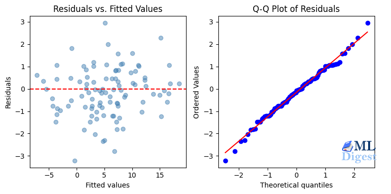
Fitting the model is only half the job. You should always inspect the residuals:
import matplotlib.pyplot as plt
from scipy import stats

residuals = y_test - y_pred_ols

fig, axes = plt.subplots(1, 2, figsize=(12, 4))

# --- Plot 1: Residuals vs. Fitted Values ---
axes[0].scatter(y_pred_ols, residuals, alpha=0.5, color="steelblue")
axes[0].axhline(0, color="red", linewidth=1.5, linestyle="--")
axes[0].set_xlabel("Fitted values")
axes[0].set_ylabel("Residuals")
axes[0].set_title("Residuals vs. Fitted Values")

# --- Plot 2: Q-Q Plot (checks normality of residuals) ---
stats.probplot(residuals, dist="norm", plot=axes[1])
axes[1].set_title("Q-Q Plot of Residuals")

plt.tight_layout()
plt.show()What you are looking for:
- Residuals vs. Fitted: points scattered randomly around the horizontal zero line, with no systematic pattern and no funnel shape.
- Q-Q plot (Quantile-Quantile plot): Q-Q plot is a scatterplot comparing the quantiles of model residuals against the quantiles of a theoretical normal distribution. Points lying close to the diagonal line indicate that the residuals are approximately Gaussian.
9. Practical Tips and Best Practices
Scale your features. Gradient descent converges much faster when all features are on a similar scale. StandardScaler (zero mean, unit variance) is the standard choice. Even for the Normal Equation, scaling makes the coefficients comparable in magnitude.
Check for multicollinearity. When two features are highly correlated (e.g., “height in cm” and “height in inches”), $\mathbf{X}^\top \mathbf{X}$ becomes near-singular, and the learned weights can be enormous and uninterpretable. The Variance Inflation Factor (VIF) is the standard diagnostic: if VIF for a feature exceeds 5–10, consider removing or combining those features.
Interpret coefficients conditionally, not causally. In a multivariate regression, the coefficient for a feature means: “holding the other included features fixed, a one-unit increase in this feature changes the prediction by this amount.” That is a conditional association, not automatically a causal effect.
Regularize by default. In practice, starting with Ridge regression almost always gives better generalization than plain OLS without a meaningful cost. Use cross-validation (e.g., RidgeCV in scikit-learn) to tune $\lambda$.
from sklearn.linear_model import RidgeCV

# Automatically tries 10 alpha values and picks the best via cross-validation (alpha is sklearn's name for our lambda)
ridge_cv = RidgeCV(alphas=np.logspace(-3, 3, 50), cv=5)
ridge_cv.fit(X_train_s, y_train)
print(f"Best alpha: {ridge_cv.alpha_:.4f}")Use the Normal Equation for small problems, gradient descent for large ones. The cutoff is roughly $d \sim 10{,}000$ features. Above that, the matrix inversion inside the Normal Equation becomes a bottleneck.
Log-transform skewed targets. If the target variable (e.g., house prices, transaction amounts) has a heavy right-skewed distribution, fitting on $\log(y)$ and then exponentiating predictions often dramatically improves RMSE and makes the residuals more Gaussian. Remember that Adjusted $R^2$ and RMSE values are then on the log scale and must be interpreted accordingly.
Separate your scaler fit from transform. A mistake that is surprisingly common: fitting the StandardScaler on the full dataset (including the test set) before the train/test split. This introduces data leakage, where the model effectively sees statistics of the test set during training. Always fit the scaler only on training data and then only transform the test data.
A Minimal Modeling Workflow
When linear regression is used in practice, the workflow matters almost as much as the equations. A disciplined sequence looks like this:
- Start with a train/validation split and a plain baseline such as predicting the mean.
- Fit an OLS or Ridge model on standardized features.
- Inspect residual plots before trusting the coefficients.
- Compare MAE, RMSE, and $R^2$ against the baseline rather than reading them in isolation.
- Only then decide whether the problem needs richer features, stronger regularization, or a non-linear model.
This order prevents a common mistake: escalating to a more complex model before checking whether the simple one failed because of data leakage, poor feature design, or a violated assumption.
When Linear Regression Is Not the Right Tool
Linear regression is a fantastic first model, but it has real limitations:
- Non-linear relationships: if a scatter plot of feature vs. target shows a clear curve, consider polynomial features, tree-based models, or neural networks.
- Classification targets: if the target is binary or categorical, use logistic regression or a classifier.
- Highly outlier-prone data: the squared loss makes linear regression sensitive to outliers. Huber regression (a robust variant) or median-based regression can be more appropriate.
- Very high-dimensional sparse data: for text features (e.g., bag-of-words with $d > 100{,}000$), sparse solvers and Lasso/Ridge are essential, and tree-based models or SVMs may outperform linear models.
That said, when in doubt, linear regression should nearly always be your baseline. If a complex model cannot substantially beat a well-tuned Ridge regression, that is a signal worth taking seriously.
Summary
Linear regression is the simplest way to learn how machine learning turns input features into predictions. It teaches you four core ideas: how a model makes a prediction, how a loss function measures error, how optimization finds good parameters, and why assumptions matter when you trust the result.
If you understand why linear regression minimizes squared error, how gradient descent or the Normal Equation finds the weights, and when regularization helps, you already understand the foundation of much of machine learning.
So what should you learn next? The next step is to explore how these ideas extend to classification problems with logistic regression, and then to more complex models like decision trees and neural networks. Each of those builds on the same core principles you have just mastered.

Silpa brings 5 years of experience in working on diverse ML projects, specializing in designing end-to-end ML systems tailored for real-time applications. Her background in statistics (Bachelor of Technology) provides a strong foundation for her work in the field. Silpa is also the driving force behind the development of the content you find on this site.

Happy is a seasoned ML professional with over 15 years of experience. His expertise spans various domains, including Computer Vision, Natural Language Processing (NLP), and Time Series analysis. He holds a PhD in Machine Learning from IIT Kharagpur and has furthered his research with postdoctoral experience at INRIA-Sophia Antipolis, France. Happy has a proven track record of delivering impactful ML solutions to clients.
Subscribe to our newsletter!