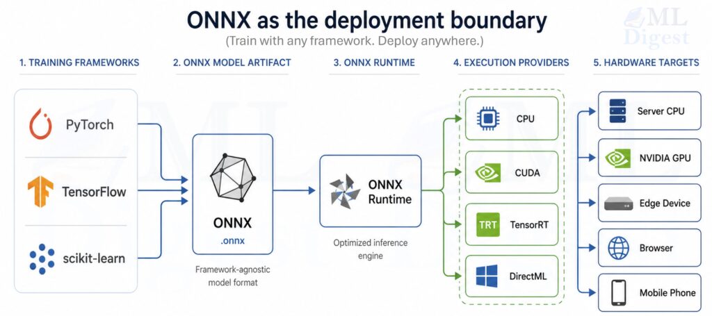
ONNX (Open Neural Network Exchange) is a standard, open-source format for representing machine learning models as a computation graph. In deployment work, ONNX is useful because it turns a training-time model into a portable inference artifact that multiple runtimes and hardware targets can execute with minimal framework-specific code.
This write-up focuses on the practical path from trained model to production inference: export, validation, optimization, packaging, and operational concerns.
If you want the broader context around where deployment fits, the machine learning project lifecycle is the larger frame in which this ONNX-specific workflow sits.
For browser-specific ONNX runtime optimization, see the ONNX Runtime Compaction guide for details on making browser ML fast and lightweight.
1. Why ONNX Deployment Matters
If training is the process of learning parameters, deployment is the process of turning those parameters into reliable, fast, and maintainable predictions in a real environment.
ONNX matters because it reduces friction at several common boundaries:
- Framework boundary: Training may be done in PyTorch or TensorFlow, while production may prefer a different runtime.
- Hardware boundary: CPUs, GPUs, and specialized accelerators have different optimal kernels.
- Platform boundary: Windows, Linux, cloud, edge, and mobile environments have different constraints and capabilities.
- Language boundary: Production services might be Python, C#, Java, C++, JavaScript, or mobile.
- Lifecycle boundary: Teams need versioning, reproducibility, CI checks, and performance regression testing.
Typical outcomes when ONNX is used well:
- Faster inference via ONNX Runtime (ORT) graph optimizations and hardware execution providers.
- Cleaner separation between model training code and inference code.
- Easier model portability and long-term maintenance.
The key idea is that ONNX is most useful when it becomes the stable artifact between model development and model serving.
In production, that artifact still belongs inside a larger MLOps loop for versioning, testing, rollout, monitoring, and rollback.
%%{init: {'theme': 'base', 'themeVariables': {
    'fontSize': '36px',
    'fontFamily': 'Arial',
    'primaryTextColor': '#000000'
}}}%%
flowchart LR
    A[Train model in PyTorch / TF / sklearn] --> B[Export to ONNX]
    B --> C[Validate: checker + parity]
    C --> D[Optimize: ORT + provider + quantize]
    D --> E[Package: model + assets + metadata]
    E --> F[Serve: API / batch / edge]
    F --> G[Monitor: latency / errors / drift]
2. ONNX Under the Hood (The Concepts That Matter in Production)
You do not need to memorize the ONNX spec to deploy models, but it helps to have the right mental model.
2.1 ONNX as a Typed Computation Graph
An ONNX model is primarily:
- A directed acyclic graph (DAG) of operators (Conv, MatMul, LayerNorm, etc.).
- Tensors flowing along edges.
- A set of initializers (usually the learned weights).
Each node has:
- An operator type (for example,
Gemm,Conv,Relu). - Attributes (for example, kernel size, strides).
- Input and output tensor names.
From a deployment perspective, this graph representation enables:
- Static analysis (shape inference, constant folding).
- Kernel selection (different implementations for CPU/GPU).
- Graph-level fusions (for example, Conv + Bias + Relu).
2.2 Opsets: Compatibility and “API Versions” for Operators
ONNX operators evolve over time. The opset version is similar to an API version for the operator set.
Best practice:
- Pin an opset version during export.
- Prefer a recent but widely supported opset (often 16–18 in current toolchains, depending on your environment).
- Test export and inference in CI so opset upgrades are deliberate.
The ONNX operator changelog documents what changed in each opset version, which is useful for diagnosing compatibility issues when upgrading tools or runtimes.
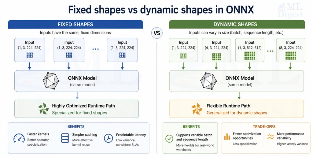
2.3 Shapes and Dynamic Axes
Deployment frequently needs flexible input sizes:
- Variable batch size
- Variable sequence length (NLP)
- Variable image size (some vision models)
ONNX can represent dynamic dimensions, but dynamic shapes may reduce optimization opportunities. A pragmatic rule:
- Make batch size dynamic almost always.
- Make sequence/image dims dynamic only when you truly need it.
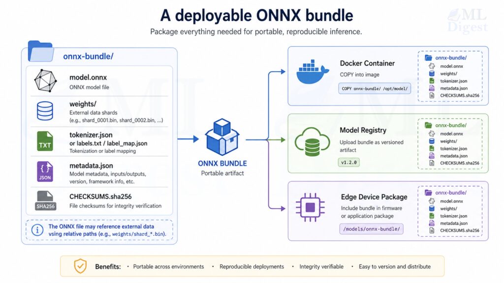
2.4 Model Size and External Data
Large models introduce a packaging concern that is easy to miss early: ONNX stores tensors either inside the protobuf itself or in external data files.
That matters in production for two reasons:
- Models with large weight sets can exceed the 2 GB protobuf size limit.
- Deployment is usually easier when the model file, weight shards, tokenizer files, and metadata are versioned as one artifact bundle.
Practical guidance:
- Treat
model.onnxplus any external weight files as a single deployable unit. - Keep external data files in stable relative locations because ONNX stores relative references.
- Validate your packaging flow in CI, not only local export, because path issues often appear first in containers or CI runners.
3. Mathematical Details That Show Up in Deployment
Most deployment bugs are not “math mistakes” in the training sense. They are usually:
- data preprocessing mismatches,
- numerical precision differences,
- shape/layout confusion,
- or quantization-induced accuracy loss.
Still, a few core mathematical ideas matter.
3.1 Numerical Parity and Tolerances
When comparing a framework model output $y$ to an ONNX output $\hat{y}$, exact equality is rarely guaranteed because of floating-point behavior and kernel differences.
You typically check that:
$$
|y – \hat{y}|_\infty \leq \varepsilon
$$
Where $\varepsilon$ depends on datatype and model sensitivity.
Practical guidance:
- FP32: start with
atol=1e-5to1e-4,rtol=1e-4. - FP16: tolerances may need to be larger.
- Quantized INT8: compare task metrics, not just raw logits.
3.2 Quantization Math (INT8 as the Main Example)
Quantization maps a float tensor $x$ into an integer tensor $q$ plus scale information.
Visual intuition (data transforms):
%%{init: {'theme': 'base', 'themeVariables': {
    'fontSize': '26px',
    'fontFamily': 'Arial',
    'primaryTextColor': '#000000'
}}}%%
flowchart LR
    X[Float tensor x] --> Q["Quantize: q = round(x/s)+z"]
    Q --> I["Int8/UInt8 tensor q"]
    Q --> P["(Store s and z)"]
    I --> DQ["Dequantize: $$\tilde{x}$$ = s*(q-z)"]
    P --> DQ
    DQ --> Y["Approx float tensor $$\tilde{x}$$"]
For affine quantization (common in ONNX Runtime), a scalar quantization can be described as:
$$
q = \mathrm{clip}(\mathrm{round}(x / s) + z, q_{\min}, q_{\max})
$$
and dequantization as:
$$
\tilde{x} = s \cdot (q – z)
$$
Where:
- $s$ is the scale (float),
- $z$ is the zero-point (integer),
- $[q_{\min}, q_{\max}]$ is typically $[-128, 127]$ for signed int8 or $[0, 255]$ for uint8.
When $z = 0$, this reduces to symmetric quantization, which is simpler and often preferred for weights. Asymmetric quantization (non-zero $z$) can represent skewed distributions more accurately and is typically better suited for activations, particularly those following a ReLU whose output range is strictly non-negative.
Important deployment implications:
- Per-channel quantization (a different scale per output channel) often preserves accuracy better for Conv/Gemm weights.
- Static quantization uses calibration data to pick scales; it often performs best but requires a calibration set.
- Dynamic quantization is simpler (commonly used for Transformer weights on CPU) but can be less accurate depending on the model.
%%{init: {'theme': 'base', 'themeVariables': {
    'fontSize': '16px',
    'fontFamily': 'Arial',
    'primaryTextColor': '#000000'
}}}%%
flowchart LR
    subgraph Dynamic Quantization
        DQ1[Quantize weights only at runtime]
    end

    subgraph Static Quantization
        SQ1[Use calibration data to compute scales]
        SQ2[Quantize weights and activations ahead of time]
    end

    subgraph Per-Channel Quantization
        PCQ1[Compute separate scale for each output channel]
        PCQ2[Preserve accuracy for Conv/Gemm layers]
    end
3.3 Latency vs Throughput (A Useful Mental Model)
If a service receives requests at rate $\lambda$ and can process at rate $\mu$, then stable operation requires roughly $\lambda < \mu$.
In practice, you control $\mu$ through:
- batching,
- model optimizations,
- execution provider choice,
- threading,
- and input size constraints.
Batching increases throughput but can increase tail latency. Deployment is usually an exercise in choosing the right trade-off for your product constraints. A common production heuristic is to set batch size as the largest value that keeps p99 latency within the service level objective, rather than optimizing for maximum throughput in isolation.
4. Exporting Models to ONNX
Export is where many long-term issues are “baked into” the artifact. The goal is to produce an ONNX model that is:
- portable,
- correct,
- and friendly to optimization.
4.1 PyTorch → ONNX (Modern and Practical)
The PyTorch ecosystem has multiple export paths. In current PyTorch ONNX exporter documentation, the recommended path is torch.onnx.export(..., dynamo=True), which uses the newer torch.export-based exporter. Older TorchScript-era flows still appear in many codebases, so you will likely encounter both.
Two patterns you will see most often are:
torch.onnx.export, withdynamo=Truein modern PyTorch, which is the main recommended exporter.- Older TorchScript-based export flows, which are still common in existing repositories and internal deployment scripts.
Below is a minimal example using the widely familiar file-based torch.onnx.export API. It is intentionally simple so the export mechanics are easy to inspect.
import torch
import torch.nn as nn


class TinyMLP(nn.Module):
    def __init__(self, in_features: int = 16, hidden: int = 32, out_features: int = 4):
        super().__init__()
        self.net = nn.Sequential(
            nn.Linear(in_features, hidden),
            nn.ReLU(),
            nn.Linear(hidden, out_features),
        )

    def forward(self, x: torch.Tensor) -> torch.Tensor:
        return self.net(x)


def main() -> None:
    torch.manual_seed(0)
    model = TinyMLP().eval()

    # Example input: dynamic batch size, fixed feature size
    x = torch.randn(2, 16)

    onnx_path = "tiny_mlp.onnx"
    torch.onnx.export(
        model,
        x,
        onnx_path,
        input_names=["input"],
        output_names=["logits"],
        dynamic_axes={"input": {0: "batch"}, "logits": {0: "batch"}},
        opset_version=17,
    )
    print(f"Exported: {onnx_path}")


if __name__ == "__main__":
main()Practical tips for PyTorch export:
- Export with
model.eval(). - Use representative input shapes.
- Name inputs and outputs explicitly.
- Prefer
dynamic_shapeswith the modern dynamo-based exporter, and usedynamic_axesmainly when maintaining older export code. - Prefer simple tensor I/O boundaries. Consider keeping complex preprocessing (text tokenization, image normalization, feature scaling) outside the ONNX model unless your deployment target supports the required operators and you want to enforce preprocessing consistency through the graph.
4.2 TensorFlow / Keras → ONNX
One common path for TensorFlow and Keras models is the tf2onnx converter. The exact commands vary depending on whether you are using a SavedModel, a Keras .h5 file, or a frozen graph. However, the deployment mindset remains consistent across all model types:
- Freeze or Save the Model: Ensure the model is in inference mode, removing training-specific operations like dropout.
- Convert to ONNX: Use the
tf2onnxtool to translate the TensorFlow operators into their ONNX equivalents while specifying the target opset. - Validate Numerically: Compare the outputs of the TensorFlow model against the resulting ONNX model using representative test data to catch any conversion discrepancies.
Example (conceptual snippet for a SavedModel):
python -m tf2onnx.convert \
  --saved-model path/to/saved_model \
  --opset 17 \
  --output model.onnx
4.3 scikit-learn → ONNX (Classical ML in Production)
Classical machine learning algorithms, including decision tree ensembles (Random Forests, Gradient Boosting), linear regression models, and composite preprocessing pipelines, can be exported using the skl2onnx library.
The key benefit is architectural uniformity: you can deploy both deep learning and classical models using a single, consistent runtime environment and artifact format. This reduces the number of dependencies required in production services and streamlines model maintenance.
!python -m pip install --upgrade torch scikit-learn skl2onnx
import numpy as np
from sklearn.datasets import load_iris
from sklearn.linear_model import LogisticRegression
from skl2onnx import convert_sklearn
from skl2onnx.common.data_types import FloatTensorType

X, y = load_iris(return_X_y=True)
clf = LogisticRegression(max_iter=200).fit(X, y)

initial_type = [("input", FloatTensorType([None, X.shape[1]]))]
onnx_model = convert_sklearn(clf, initial_types=initial_type, target_opset=17)

with open("iris_lr.onnx", "wb") as f:
    f.write(onnx_model.SerializeToString())

print("Exported: iris_lr.onnx")5. Validating Correctness (Before You Optimize)
Validation must be routine and heavily automated. Relying on visual checks or ad hoc script runs exposes the deployment pipeline to regressions, particularly when updating opset versions, changing execution providers, or migrating across environments.
That is the same mindset behind testing machine learning: use small automated checks that fail early when model behavior changes.
5.1 Structural Checks
Use ONNX tooling to ensure the graph itself is structurally sound. Structural validation confirms that operator types are recognized, attributes conform to the spec, tensor types are internally consistent, and the serialized graph is well-formed. It does not guarantee runtime behavior on a specific execution provider, which is why numerical parity checks (see section 5.2) remain mandatory.
!python -m pip install --upgrade onnx onnxruntime numpy
import onnx

model = onnx.load("tiny_mlp.onnx")
onnx.checker.check_model(model)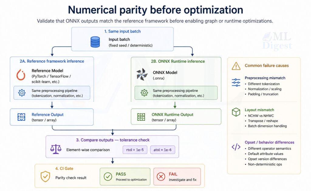
print("ONNX model is structurally valid")5.2 Numerical Parity Checks with ONNX Runtime
This is the most important practical check: run the ONNX model and compare to a reference.
import numpy as np
import onnxruntime as ort
import torch
import torch.nn as nn


class TinyMLP(nn.Module):
    def __init__(self, in_features: int = 16, hidden: int = 32, out_features: int = 4):
        super().__init__()
        self.net = nn.Sequential(
            nn.Linear(in_features, hidden),
            nn.ReLU(),
            nn.Linear(hidden, out_features),
        )

    def forward(self, x: torch.Tensor) -> torch.Tensor:
        return self.net(x)


def main() -> None:
    torch.manual_seed(0)
    np.random.seed(0)

    model = TinyMLP().eval()
    x = torch.randn(8, 16)

    # Reference output
    with torch.no_grad():
        ref = model(x).cpu().numpy()

    sess = ort.InferenceSession("tiny_mlp.onnx", providers=["CPUExecutionProvider"])
    ort_out = sess.run(None, {"input": x.cpu().numpy()})[0]

    np.testing.assert_allclose(ref, ort_out, rtol=1e-4, atol=1e-4)
    print("Parity check passed")


if __name__ == "__main__":
main()If parity fails, the most common causes are:
- Export produced a different graph (for example, training-only behavior was not disabled).
- Preprocessing or tokenization differs.
- Data layout differs (NCHW vs NHWC).
- Unsupported operator behavior differs across opsets.
6. Performance Optimization with ONNX Runtime
Optimization is usually done after correctness is established. Starting from an unverified baseline makes it difficult to distinguish optimization-induced accuracy regressions from pre-existing export bugs. The main levers are graph-level transformations applied by ORT, execution provider selection for hardware-specific kernels, and quantization to reduce model size and arithmetic cost.
6.1 Use Graph Optimizations
ONNX Runtime can apply graph optimizations when creating the session.
Conceptually, think of ORT as doing “compiler passes” on the graph:
- constant folding,
- operator fusions,
- layout transformations,
- memory planning.
import onnxruntime as ort

so = ort.SessionOptions()
so.graph_optimization_level = ort.GraphOptimizationLevel.ORT_ENABLE_ALL

sess = ort.InferenceSession("tiny_mlp.onnx", sess_options=so, providers=["CPUExecutionProvider"])6.2 Pick the Right Execution Provider
Execution providers are the bridge from the ONNX graph to hardware-specific kernels.
Common providers:
- CPUExecutionProvider: most portable, good baseline.
- CUDAExecutionProvider: NVIDIA GPU.
- TensorRTExecutionProvider: NVIDIA TensorRT (often best for latency/throughput when compatible).
- DirectMLExecutionProvider: Windows GPU acceleration on some setups.
The full list of supported execution providers is available in the ONNX Runtime documentation.
Practical advice:
- Start with CPU, then test CUDA/TensorRT if latency is important.
- Keep a CPU fallback in case a GPU provider fails to load.
- Treat provider choice as a deploy-time configuration, not a code change.
6.3 Quantization (Often the Highest ROI on CPU)
Quantization can reduce model size and improve CPU latency substantially. The ONNX Runtime quantization documentation covers all supported modes and calibration options in detail.
6.3.1 Dynamic Quantization (Simple)
In dynamic quantization, weights are quantized ahead of time, but activations are quantized on the fly during inference. This is often a good first step for CPU models because it is simple and does not require a calibration dataset.
from onnxruntime.quantization import QuantType, quantize_dynamic, quant_pre_process

quant_pre_process("tiny_mlp.onnx", "tiny_mlp.preprocessed.onnx") # quant_pre_process cleans up the model's shape information (runs graph optimizations and fixes shape annotations)
quantize_dynamic(
    model_input="tiny_mlp.preprocessed.onnx",
    model_output="tiny_mlp.int8.onnx",
    weight_type=QuantType.QInt8,
)
print("Wrote: tiny_mlp.int8.onnx")Dynamic quantization is commonly effective for linear layers and Transformer-style models on CPU.
6.3.2 Static Quantization (More Work, Often Better)
Static quantization uses a calibration dataset to estimate activation ranges ahead of time, which often produces more accurate quantized models than dynamic quantization because activation scale factors are determined from representative data rather than inferred at runtime.
Deployment pattern:
- Collect calibration samples that represent the full distribution of production inputs. The diversity and representativeness of the calibration set matters more than its size; typically 100 to 500 samples is sufficient for most models, but a narrowly chosen set can degrade accuracy even at higher counts.
- Implement a
CalibrationDataReaderthat feeds these samples to ORT’s calibration pass. - Run the calibration pass to compute per-tensor or per-channel activation scales.
- Produce an INT8 model.
- Validate task metrics (accuracy, F1, BLEU, and so on) against the FP32 baseline, not just raw output values.
- Benchmark latency and confirm the reduction meets your requirements.
6.4 FP16 Conversion (Common on GPUs)
FP16 often helps on GPUs when the provider supports fast half-precision kernels. You can convert an existing FP32 ONNX model to FP16 using the convert_float_to_float16 utility from onnxconverter-common. Note that not all operators support FP16 natively; the runtime falls back to FP32 for unsupported nodes, so the end-to-end latency gain depends on operator coverage in the graph.
Treat FP16 as a separate artifact with its own validation and monitoring, because numerical behavior can change and overflow is possible for activations with large magnitude.
7. Implementation Steps: A Practical End-to-End Checklist
This section is written like a repeatable operating procedure rather than a one-time migration checklist.
7.1 Export
- Set the model to inference mode (
eval()for PyTorch). - Choose a stable opset.
- Decide which dimensions must be dynamic.
- Name inputs and outputs.
- Export and store the ONNX file as a versioned artifact.
Artifacts to keep together:
model.onnx- label maps, tokenizer files, or normalization statistics
- a small metadata file (model version, opset, input schema)
7.2 Validate
onnx.checker.check_model- Run a parity check on a small batch of representative inputs.
- Add a CI job that fails if parity is broken.
7.3 Optimize
- Enable ORT graph optimizations.
- Select provider (CPU, CUDA, TensorRT, DirectML) based on environment.
- Evaluate quantization (dynamic first, then static if needed).
- Benchmark latency and throughput.
7.4 Package
- Bundle the ONNX model and auxiliary assets.
- Ensure you have a reproducible environment (Docker, pinned dependencies).
- Add a startup self-test: load the model, run a tiny inference, and fail fast if broken.
7.5 Serve
- Warm up the model session.
- Control concurrency and threading.
- Log latency and failures.
- Add monitoring for input anomalies and drift.
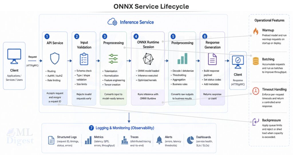
8. Serving Patterns (What Works Well in Real Systems)
This section avoids framework-specific “extra features” and focuses on reliable patterns.
8.1 Python Microservice (Common Baseline)
Common best practices when using ORT in a service:
- Create the
InferenceSessiononce at process startup. - Avoid re-loading the model per request.
- Validate and normalize inputs explicitly.
- Keep preprocessing consistent with training.
Minimal skeleton (illustrative):
import numpy as np
import onnxruntime as ort

class OnnxPredictor:
    def __init__(self, model_path: str) -> None:
        so = ort.SessionOptions()
        so.graph_optimization_level = ort.GraphOptimizationLevel.ORT_ENABLE_ALL
        # Common knobs to consider in production:
        # so.intra_op_num_threads = 1
        # so.inter_op_num_threads = 1
        # so.execution_mode = ort.ExecutionMode.ORT_SEQUENTIAL
        self.sess = ort.InferenceSession(model_path, sess_options=so, providers=["CPUExecutionProvider"])
        self.input_name = self.sess.get_inputs()[0].name

    def predict(self, x: np.ndarray) -> np.ndarray:
        out = self.sess.run(None, {self.input_name: x})[0]
return outOperational tips:
- For CPU inference, tune ORT threading depending on your workload and core count.
- Consider batching if you have high request volume.
- Use timeouts and backpressure so the service degrades gracefully.
8.2 Batch Inference Jobs
ONNX is also well-suited to batch scoring:
- Load model once.
- Stream data in chunks.
- Write predictions to a data store.
Batch jobs often benefit more from throughput optimizations (bigger batches) than from tail-latency optimizations.
8.3 Edge, Mobile, and Browser
Constraints shift on-device:
- Memory is limited.
- Startup time matters.
- Hardware acceleration availability varies.
Common approaches:
- ONNX Runtime Mobile: Pre-built, size-optimized builds for Android and iOS. If binary size matters, use ONNX Runtime’s reduced operator configuration and custom build flow to include only the operators your model requires.
- onnxruntime-web: Browser inference via WebAssembly or WebGPU. WebAssembly provides broad cross-browser compatibility; WebGPU enables GPU-accelerated inference on supported browsers with significantly better throughput for larger models.
Practical guidelines for edge and mobile deployments:
- Keep the ONNX artifact small. INT8 quantization reduces weight storage from 4 bytes (FP32) to 1 byte, yielding roughly 4x size reduction for weight-dominated models.
- Prefer compact architectures (such as MobileNet or EfficientNet variants, or distilled models) when designing for constrained targets from the start.
- Test on representative target hardware early. Inference speed and operator support can differ substantially between emulators and physical devices.
- Minimize the runtime as well as the model. On mobile, runtime binary size can matter almost as much as model size.
9. Best Practices (The Short List That Prevents Most Pain)
9.1 Export Hygiene
- Pin opset version.
- Keep I/O schemas stable and documented.
- Prefer explicit preprocessing steps and version them.
- Keep a “golden set” of test inputs and outputs for regression tests.
9.2 Correctness and Regression Testing
- Add parity checks to CI for at least a small sample set.
- Test on the same execution provider you deploy (CPU vs GPU).
- Treat quantized and FP16 models as separate artifacts with separate tests.
9.3 Performance Engineering
- Benchmark with realistic input sizes and batch sizes.
- Measure p50, p95, and p99 latency, not only average.
- Prefer provider-specific optimization paths only after a stable baseline exists.
9.4 Observability and Operations
- Log model version, provider, and latency.
- Monitor errors and timeouts.
- Add drift indicators where appropriate (feature distribution shifts, embedding norms, etc.).
9.5 Security and Supply Chain
- Treat the ONNX model as untrusted input unless it is produced by your pipeline. A malicious ONNX file could contain operators or attributes crafted to exploit parser vulnerabilities during loading.
- Verify hashes (SHA-256 or stronger) for model artifacts at both download time and load time.
- Pin ORT and conversion tool versions in your dependency manifest and lock file to prevent silent behavior changes from upstream updates.
- Store model artifacts in a controlled registry with access logging rather than in public object storage, unless public access is intentional and the artifact is verified.
10. Common Failure Modes and How to Debug Them
Most ONNX deployment failures fall into a small set of repeating categories. Recognizing the symptom pattern early significantly reduces debugging time.
10.1 Unsupported or Differently-Defined Operators
Symptoms:
- Export fails.
- ORT fails to load.
- Parity fails badly.
Actions:
- Try a different opset.
- Simplify the model or replace unsupported layers.
- Check whether the execution provider supports the required operators.
10.2 Layout Mismatches (NCHW vs NHWC)
Symptoms:
- Outputs are wrong but not random.
- Accuracy collapses.
Actions:
- Confirm tensor shapes and layout conventions end-to-end.
- Ensure preprocessing matches what the model expects.
10.3 Preprocessing and Tokenization Drift
Symptoms:
- Model seems correct on some inputs but fails in production.
Actions:
- Version preprocessing assets (tokenizers, vocab, normalization statistics).
- Add input schema validation.
- Consider exporting preprocessing into the model only if it is stable and supported.
10.4 Dynamic Shapes Causing Performance Surprises
Symptoms:
- Correct outputs but poor performance.
Actions:
- Constrain dynamic dimensions if possible.
- Consider exporting multiple models for common shapes.
- Profile provider-specific behavior.
10.5 Large Models and Packaging Failures
Symptoms:
- The model exports successfully but fails after packaging or containerization.
onnx.checkerworks locally but not in CI.- Runtime loading fails because weight files cannot be found.
Actions:
- If the model uses external data, package the
.onnxfile and its external tensor files together. - For models larger than 2 GB, run
onnx.checker.check_modelon the model path rather than only on an in-memory object. - Verify relative paths after copying artifacts into Docker images, model registries, or edge bundles.

Silpa brings 5 years of experience in working on diverse ML projects, specializing in designing end-to-end ML systems tailored for real-time applications. Her background in statistics (Bachelor of Technology) provides a strong foundation for her work in the field. Silpa is also the driving force behind the development of the content you find on this site.

Happy is a seasoned ML professional with over 15 years of experience. His expertise spans various domains, including Computer Vision, Natural Language Processing (NLP), and Time Series analysis. He holds a PhD in Machine Learning from IIT Kharagpur and has furthered his research with postdoctoral experience at INRIA-Sophia Antipolis, France. Happy has a proven track record of delivering impactful ML solutions to clients.
Subscribe to our newsletter!