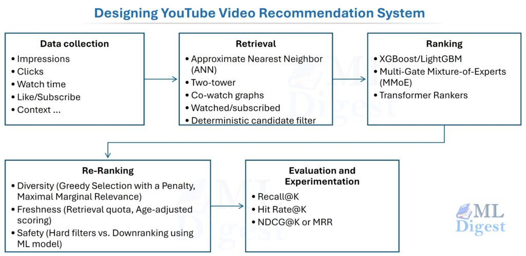
This article is a system-design blueprint for a YouTube-like recommender: how it serves results in milliseconds, how it learns from noisy implicit feedback, and how it stays reliable under scale, freshness, and safety constraints.
1. Introduction: The Library of Billions
At YouTube scale, the central problem is not storing videos. It is deciding, in a few hundred milliseconds, which handful of videos from a catalog of billions should appear for one specific user at one specific moment.
Public papers reveal the main patterns, but not the exact production implementation. This article is therefore a technically grounded blueprint for a YouTube-like system, not a claim about YouTube’s internal stack.
You cannot run a heavy, complex neural network on a billion videos in milliseconds. Instead, you must reduce the universe of content in stages, spending more computational power as the pool gets smaller. That multi-stage funnel is the defining architectural pattern of modern recommendation systems.
Recommendation quality drives user satisfaction, creator discovery, platform safety, and long-term retention. The engineering challenge is that the system must operate at high Queries Per Second (QPS), stay fresh, support continuous model updates, and learn from biased, delayed feedback.
1.1 The Theoretical Foundation
Public understanding of YouTube-style recommenders largely comes from a few Google papers. Covington et al. (2016) established the two-stage pattern of candidate generation plus ranking. Zhao et al. (2019) showed the shift from click-only optimization toward multi-task objectives such as clicks, watch time, and negative feedback. Ma et al. (2018) formalized MMoE, now a common ranking architecture for balancing those tasks.
1.2 Problem Statement and Constraints
At a high level, the request-time problem is:
Given a user $u$ in context $c$ (surface, device, language, session state) and a universe of items $\mathcal{I}$, return a ranked list of $K$ items that maximizes long-term user satisfaction subject to safety and product constraints.
In practice, this becomes a constrained optimization problem under strict service-level objectives (SLOs):
- Latency: optimize p99 end-to-end latency, not average latency.
- Freshness: new uploads and rapidly shifting user intent must be reflected quickly.
- Safety and policy: certain items must be filtered or downranked deterministically.
- Reliability: the system must degrade gracefully under partial outages.
- Experimentation: the serving stack must support controlled exploration and reproducible A/B tests.
2. High-level Architecture (What happens on one request)
The request path is a staged funnel that narrows billions of videos to a small final slate. Early stages optimize recall under tight latency budgets; later stages spend more compute on precision and policy enforcement.
flowchart LR
    %% Nodes
    A["BILLIONS OF VIDEOS<br/><br/>All Available Content"]
    B["Candidate Generation<br/><br/>1,000 – 50,000 Videos"]
    C["Ranking<br/><br/>Few Hundred Videos"]
    D["Re-ranking<br/><br/>10 – 20 Videos<br/>Shown on Screen"]

    %% Flow
    A ==> B
    B ==> C
    C ==> D

    %% Styling (wide → narrow effect via color emphasis)
    style A fill:#1f77b4,color:#ffffff,stroke:#0d3b66,stroke-width:3px
    style B fill:#2a9df4,color:#ffffff,stroke:#0d3b66,stroke-width:2px
    style C fill:#6ec6ff,color:#000000,stroke:#0d3b66,stroke-width:2px
    style D fill:#cfe9ff,color:#000000,stroke:#0d3b66,stroke-width:2px
Each stage has a distinct job and budget:
- Retrieval (Candidate Generation): Select a few thousand plausible videos from billions. Must execute in tens of milliseconds. It prioritizes high recall (making sure the good stuff is in the pool) over precision.
- Ranking: Takes tens to low hundreds of milliseconds. It uses heavy features and complex models to achieve high precision.
- Post-processing (Re-ranking): Must be deterministic, lightning-fast, and auditable to apply business rules and safety constraints.
2.1 Core Components of the System
The following diagram illustrates the lifecycle of data and models across the full system. User interactions produce training signals, which feed back into the training pipelines, which update the serving models and feature store — a continuous feedback loop where each component depends on the health of the others.
%%{init: {'theme': 'base', 'themeVariables': {
    'fontSize': '22px',
    'fontFamily': 'Arial',
    'primaryTextColor': '#000000'
}}}%%

flowchart LR

    %% =====================
    %% Core Components
    %% =====================

    A["<b>Data Collection & Logging</b><br/><br/>
    • Impressions<br/>
    • Clicks / Watch Time<br/>
    • Like / Subscribe / Comment / Skip <br/>
    • Context (device, language, time)<br/>
    • Session State"]

    B["<b>Offline Training Pipelines</b><br/><br/>
    • Feature Engineering<br/>
    • Embeddings<br/>
    • Train Retrieval & Ranking Models"]

    C["<b>Online Feature Store</b><br/><br/>
    • Low-Latency Feature Access<br/>
    • User & Item Features<br/>
    • Offline/Online Parity"]

    D["<b>Online Serving</b><br/><br/>
    • ANN Index (Embeddings)<br/>
    • Model Servers (Rankers)<br/>
    • Caches"]

    E["<b>Experimentation & Monitoring</b><br/><br/>
    • A/B Testing<br/>
    • Guardrails<br/>
    • Drift Detection<br/>
    • Data Quality Checks"]

    %% =====================
    %% Data Flow
    %% =====================

    A --> B
    B --> C
    C --> D
    D --> A
    D --> E
    E --> B

    %% =====================
    %% Styling
    %% =====================

    style A fill:#1f77b4,color:#ffffff,stroke:#0d3b66,stroke-width:2px
    style B fill:#2a9df4,color:#ffffff,stroke:#0d3b66,stroke-width:2px
    style C fill:#6ec6ff,color:#000000,stroke:#0d3b66,stroke-width:2px
    style D fill:#a8dadc,color:#000000,stroke:#0d3b66,stroke-width:2px
    style E fill:#f1faee,color:#000000,stroke:#0d3b66,stroke-width:2px
Each component has a clear role:
- Data Collection & Logging records impressions, engagement, and context as immutable events.
- Offline Training Pipelines turn those logs into features, and new model checkpoints.
- Online Feature Store serves low-latency features while preserving offline/online parity.
- Online Serving retrieves, ranks, and returns results under strict latency budgets.
- Experimentation & Monitoring runs A/B tests, tracks guardrails, and detects regressions or drift.
2.2 Recommendation Surfaces and Context
“Recommendation” is not one endpoint. Different surfaces have different intents and constraints:
- Home feed: broad discovery and re-engagement; strong diversity and long-term satisfaction constraints.
- Up Next: short-term intent and sequence continuation; stronger emphasis on session-level objectives.
- Shorts feed: extremely short feedback loops; position bias and skip signals become dominant.
- Search suggestions: explicit query intent; lexical and semantic matching matter more than long-term preferences.
A practical design keeps the overall architecture shared but allows surface-specific retrieval sources, ranking features, re-ranking rules, and exploration rates.
3. Data, Signals, and Objectives
Recommendation is not just about “predicting a click”. A typical system predicts and optimizes for a mix of objectives to ensure long-term health.
- Click probability (estimated CTR)
- Expected watch time, optionally conditioned on click
- Satisfaction proxies: likes, long watches, and survey signals
- Negative outcome probability: quick skips, “not interested” taps, and reports
3.1 The Logging Contract (What must be logged)
Most recommendation failures are data failures. If the logging contract is incomplete, training becomes biased and debugging becomes guesswork.
At minimum, every served list should be reconstructible from logs. That requires logging not only the user action, but also what the system decided to show.
Here is a minimal impression-level schema (conceptual, not tied to a specific storage technology):
impression_id            unique id for this impression event
request_id               groups impressions served together
timestamp_ms             event time

user_id                  stable user id (or anonymous id)
surface                  home | up_next | shorts | search
device                   mobile | desktop | tv
locale                   language/region

item_id                  video id
rank_position            integer position in the served list

retrieval_sources        list of sources that retrieved the item (ann, subscriptions, covisitation, trending)
model_versions           retrieval_model_version, ranker_version, reranker_version
experiment_ids           active experiment/bucket ids

propensity               probability of being shown (or a proxy), for counterfactual evaluation
served_score             score used at serve time (optional, but helpful for audits)

click                    0/1
watch_time_ms            dwell/watch duration
liked, shared, reported  0/1 signals
subscribed               0/1 (user subscribed to the video's channel)
commented                0/1 (and optionally comment_length_chars as a depth signal)
Several details matter disproportionately in practice:
- Impressions are first-class events. Training on clicks alone guarantees exposure bias.
- Model versions and experiment IDs are non-negotiable. Without them, it is impossible to reproduce “why was this shown?” and to perform clean offline-to-online comparisons.
- User identifiers must be privacy-safe. Stable user IDs should never appear raw in training data or logs that are stored long-term. Rotate or hash pseudonymous IDs consistently, apply retention windows to raw event logs, and ensure that any personally identifiable information (PII) is stripped or tokenized before it passes through the training pipeline. Compliance with data-retention regulations (GDPR, CCPA) starts here, at the logging contract level.
3.2 Signal Quality and the Training Data Contract
User feedback comes in two forms. Implicit feedback such as impressions, clicks, and watch time is dense but noisy. Explicit feedback such as likes, subscribes, reports, and comments is sparse but higher quality. Both matter, but neither comes from a neutral sample of content.
3.3 Key Sources of Bias and Mitigation Strategies
Recommendation data is structurally biased. Five common issues appear in most production systems:
- Exposure bias occurs because we only observe user feedback on the tiny fraction of videos we actually show them. The model never sees evidence of what users would have done had they been offered a different set of choices.
- Position bias skews our understanding of relevance: users naturally click on the top-ranked items simply because they are at the top, not because those items are inherently better. A click on position 1 carries a very different meaning than a click on position 10.
- Selection bias creates a feedback loop where the system’s past decisions dictate the training data for its future self — a model that ranks action videos highly generates more action-video data, reinforcing its own beliefs.
- Popularity amplification (feedback loops): at scale, even a small preference for popular items compounds over time, concentrating traffic on a shrinking set of viral content and crowding out everything else.
- Policy and safety censoring: filtered or removed items disappear entirely from the logs. Unless the removal reason is recorded, the training distribution silently shifts in ways that are hard to diagnose.
The following table summarizes the primary mitigation for each:
| Bias | Root Cause | Primary Mitigation |
|---|---|---|
| Exposure | Only labeled what we showed | Log impressions as first-class events; use exploration traffic |
| Position | Higher positions get more clicks regardless of quality | Log rank position; apply IPS or explicit examination models |
| Selection | Model reinforces its own past decisions | Randomized buckets; exploration holdouts |
| Popularity amplification | Popular items generate more data | Inverse frequency weighting; discovery lanes (Section 8.3) |
| Safety censoring | Filtered items leave no trace | Log removal reason codes; track filtered-item distribution |
Techniques like Inverse Propensity Scoring (IPS) can partly correct for exposure bias when the logging policy is understood. Position bias usually requires explicit examination modeling or a dedicated debiasing step rather than simply adding rank as a feature.
4. Candidate Generation (Retrieval)
Candidate generation answers a fundamental question: “Which few thousand videos are worth ranking?”
At this stage, we prioritize speed and recall. The goal is not perfect ordering, only a pool that likely contains the good answers. In practice, that requires multiple retrieval sources.
One concrete way to think about retrieval is as a union of “candidate lanes” with quotas:
flowchart LR
    U[User + Context] --> A[ANN / Two-Tower]
    U --> B[Co-watch Graph]
    U --> C[Subscriptions]
    U --> D[Trending / Fresh]
    U --> E[Query/Topic Retrieval]

    A --> M[Union + De-dup + Quotas]
    B --> M
    C --> M
    D --> M
    E --> M

    M --> F[Cheap Filters]
    F --> R[Ranking]
This pattern keeps recall high while preventing any single source from dominating the pool.
4.1 Retrieval Sources in Practice: Beyond Embeddings
Two-tower retrieval is usually combined with other high-recall sources: co-watch graphs, subscriptions and channel affinity, similar-to-recently-watched, trending or fresh content, and topic or query retrieval. The system unions these lanes, deduplicates results, and applies per-source quotas so one source does not dominate. Those quotas are usually surface-specific: Home favors discovery, while Up Next favors session continuity.
- The co-watch graph finds videos frequently watched together (“users who watched X also watched Y”). This captures the “wisdom of the crowd”—if thousands of users who watched a specific physics lecture also watched a particular calculus tutorial, the system learns a semantic link that deep neural networks might miss in the early stages of training.
- Fetching videos similar to recently watched content captures short-term session intent.
- User’s subscriptions and channel affinities are high-precision signals. They capture explicit user intent.
- Contextual candidates like local trending videos or breaking news are independent of the user’s history but highly relevant to the “now.”
- Topic-based retrieval is used for specific search queries, ensuring that the pool of candidates is grounded in the explicit keywords provided by the user.
In production, teams usually make these caps explicit and surface-specific. For example, Home may reserve more quota for discovery sources, while Up Next may reserve more quota for “similar to recently watched” and session-based sources.
4.2 The Two-Tower Architecture: Connecting Users and Content
The Two-Tower architecture maps users and videos into the same embedding space so similarity can be computed efficiently.
- The User Tower: A neural network that takes everything we know about the user (watch history, search queries, demographics) and compresses it into a single dense vector—the coordinates of the user.
- The Item Tower: A separate neural network that takes everything we know about the video (title, tags, thumbnail features) and compresses it into a vector of the exact same size—the coordinates of the video.
Because both live in the same space, compatibility is measured by dot product or cosine similarity. Specialized nearest-neighbor indexes make this much cheaper than brute-force scanning.
4.2.1 Mathematical Formulation and Training
Let $f_\theta(u,c) \in \mathbb{R}^d$ be the user embedding generated by the user tower with parameters $\theta$, and $g_\phi(i) \in \mathbb{R}^d$ be the item (video) embedding generated by the item tower with parameters $\phi$. Both vectors have dimension $d$.
The predicted relevance score is the inner product of these two vectors:
$$
s(u,i,c) = f_\theta(u,c)^\top g_\phi(i)
$$
To train these towers, we treat “the next watched video” as the positive target $i^+$. We also need negative examples $i^-_j$ (videos the user did not watch) so the model learns what to push away from. This is a form of Contrastive Learning.
A highly effective approach is using the InfoNCE loss (often implemented as an in-batch softmax with temperature scaling). For a given user $u$, positive item $i^+$, a set of negative items ${i^-_j}$ sampled from the batch, and a temperature parameter $\tau$, the loss function is:
$$
\mathcal{L} = -\log \frac{\exp(s(u,i^+,c)/\tau)}{\exp(s(u,i^+,c)/\tau) + \sum_j \exp(s(u,i^-_j,c)/\tau)}
$$
This loss function forces the score for the positive video $s(u,i^+,c)$ to be significantly larger than the scores of the negative videos. The temperature $\tau$ controls the sharpness of the distribution, scaling the penalization of hard negatives.
Precision often improves further with hard negative mining, where negatives are chosen from items the model scores highly but the user ignored. Including these during training forces the model to learn the fine-grained differences between “relevant” and “almost relevant” content.
4.2.2 Sequence-Aware User Tower
User history is ordered, so the user tower is often made sequence-aware. A simple version pools recent item embeddings; stronger versions use GRUs or Transformers over the last $T$ events, optionally with time-gap and surface features.
4.3 Approximate Nearest Neighbor (ANN) Serving
With item embeddings $g_\phi(i)$ computed for all videos, retrieval mathematically becomes a maximum inner product search:
$$
\text{TopK}(u) = \arg\max_{i \in \mathcal{I}} f_\theta(u,c)^\top g_\phi(i)
$$
Because $|\mathcal{I}|$ is huge, exact search is infeasible. Approximate Nearest Neighbor (ANN) indexes such as HNSW (Hierarchical Navigable Small World graphs) or IVF-PQ (Inverted File with Product Quantization) trade a small amount of recall for large latency savings. Production systems often shard indexes by language or region, quantize embeddings, and maintain a smaller fresh index alongside a stable main index.
Three operational details matter:
- Index consistency and versioning: user embeddings and item embeddings must be compatible (same dimension, normalization, training recipe). Rolling out new embedding models typically requires dual-writing embeddings and serving from multiple indexes during migration.
- Deletes and policy filters: item removals (copyright, safety, private videos) must propagate quickly. Many systems implement “tombstones” or fast filter layers in front of the ANN results.
- Freshness vs. stability: frequent index rebuilds improve freshness but can hurt cache locality and make debugging harder. A common compromise is a stable main index plus a smaller, rapidly updated fresh index.
4.4 Candidate Filtering Before Ranking
Before passing candidates to the ranking models, we apply a layer of cheap, deterministic filters. This step prunes the pool by removing blocked videos, enforcing age restrictions, and filtering out items the user has already watched. We also perform deduplication to ensure that if multiple sources suggested the same video, it only occupies one slot in the ranking queue.
5. Ranking Models (Precision)
Retrieval answers, “What is worth considering?” Ranking answers the harder question: “Among these candidates, what should appear first for this user right now?”
This is where most modeling sophistication lives. The ranker uses richer context to balance user preference, session intent, freshness, and long-term satisfaction.
5.1 Comprehensive Feature Sets
The ranker’s precision comes from the breadth and quality of its features.
- User Features: Language, geography, device type, and recent session statistics (e.g., number of videos watched in the last hour).
- Item Features: Topic, channel, upload age, and historical engagement rates (CTR, completion rate).
- User-Item Cross Features: Historical affinity for the video’s channel or the overlap between the video’s tags and the user’s long-term interests.
- Contextual Features: Time of day, day of the week, or the specific UI surface being used.
In practice, the hard part is not inventing features but computing and joining them under latency constraints. That is why the feature store and cache strategy are part of the ranker design.
5.2 Model Families: From Trees to Transformers
When choosing a model architecture, the main trade-off is predictive power versus serving cost.
Gradient Boosted Decision Trees (GBDTs) such as XGBoost or LightGBM are strong baselines for tabular features and fast inference, but they are less natural for very high-cardinality sparse IDs.
To handle sparse IDs alongside dense features, we use deep learning architectures:
- Wide & Deep (Cheng et al., 2016): This model jointly trains a wide component (a linear model over manually engineered cross-features) with a deep component (a feed-forward network over learned embeddings). The wide side memorizes specific co-occurrence patterns (e.g., a known user-item affinity pair); the deep side generalizes to unseen combinations. The two components share a single final output layer.
- DeepFM (Guo et al., 2017): A refinement that replaces the wide component’s manual feature crossing with a Factorization Machine (FM) layer. This removes the need for expert-crafted cross-feature sets, letting the model discover second-order interactions automatically and making it easier to deploy across new feature domains.
- Transformer Rankers: These models treat the user’s session as a sequence, using self-attention to weigh the importance of past interactions when scoring the current candidate. They excel at capturing long-range positional context but require more careful latency budgeting than the shallower alternatives.
5.3 Multi-Task Learning: Multi-Gate Mixture-of-Experts (MMoE)
A modern ranker does not just predict one thing. Following the shift away from purely CTR-driven optimization (which fostered clickbait), systems must simultaneously optimize opposing metrics like expected watch time and the likelihood of explicitly liking a video versus the probability of negative feedback like skipping within seconds.
Traditional “shared-bottom” architectures pass all features through a common set of layers before splitting into task-specific heads. However, this often leads to negative transfer or task interference, where a task with sparse data (e.g., sharing a video) is “overwhelmed” by the gradient of a task with dense data (e.g., clicking) because they compete for the same representational capacity in the shared layers.
To solve this, Google researchers introduced the Multi-Gate Mixture-of-Experts (MMoE) architecture, which decoupled the rigid shared-bottom constraint. This approach consists of:
- Multiple Shared Experts: A set of $n$ expert networks ${e_1, e_2, \dots, e_n}$ that process the input.
- Task-Specific Gates: For each task $k$, a gate function $g^k(x)$ (typically a softmax) that outputs a weighting vector:
$$
g^k(x) = \text{softmax}(W_{gk}x)
$$ - Task Output: The final representation for task $k$ is an attention-weighted sum of the expert outputs:
$$
f^k(x) = \sum_{j=1}^n g^k_j(x) e_j(x)
$$
This allows the model to learn complex relationships: one gate might prioritize “content” experts for watch time, while another gate might focus on “creator affinity” experts for likes. By allowing each task to focus on its own optimal blend of experts, MMoE reduces interference and significantly improves multi-task performance.
At serving time, these task heads are not used as separate product decisions. Instead, the system converts them into calibrated estimates such as click probability, expected watch time, like probability, and bad-outcome probability, then combines them into a single ranking score that can be sorted efficiently before later re-ranking constraints are applied.
5.4 Loss Functions: Pointwise, Pairwise, and Listwise
Rankers are typically trained with one of three loss families.
5.4.1 Pointwise (Classification and Regression)
The simplest approach is to look at one video at a time. For clicks ($y \in {0, 1}$), we use the Binary Cross-Entropy (Logistic Loss). This is equivalent to maximizing the likelihood of a Bernoulli distribution for each impression:
$$
\mathcal{L}_{\text{logloss}} = -y\log(p) – (1-y)\log(1-p)
$$
For watch time, we use a regression loss like Mean Squared Error (MSE) on the logarithm of the duration. While stable, pointwise losses do not explicitly optimize for the relative order of items, which can be a drawback for ranking.
5.4.2 Pairwise Ranking
Pairwise ranking focuses on the relative order: it learns that a positive item should score higher than a negative one. This is the core idea behind architectures like RankNet. The loss function encourages the margin between the two scores to be as large as possible:
$$
\mathcal{L}_{\text{pair}} = -\log\sigma(\hat{s}(u,i^+) – \hat{s}(u,i^-))
$$
Extensions such as LambdaRank and LambdaMART build on this idea by scaling the pairwise gradient by the change in NDCG that would result from swapping the pair, providing a more direct connection between the training objective and the final ranking metric without requiring NDCG to be directly differentiable.
5.4.3 Listwise and NDCG
In the final evaluation, we care about the entire list. Normalized Discounted Cumulative Gain (NDCG) is the gold standard, as it penalizes the model more for making mistakes at the top of the list than at the bottom:
$$
\text{NDCG@K} = \frac{1}{\text{IDCG@K}}\sum_{k=1}^K \frac{2^{\text{rel}_k}-1}{\log_2(k+1)}
$$
Here, $\text{rel}_k$ is graded relevance and $\text{IDCG@K}$ normalizes against the ideal ordering. Listwise training can improve top-of-list quality, but it is harder to implement and debug.
5.5 Calibration: Ensuring Score Reliability
A ranker might output a score of 0.8, but does that mean there is an 80% chance of a click? In production, we need the scores to be well-calibrated. If our model predicts an 80% CTR for a group of videos, we should observe roughly 80 clicks for every 100 impressions.
We achieve this through Platt Scaling or Isotonic Regression. Calibration is crucial because it allows us to combine scores from different models (e.g., combining a click probability with a watch-time estimate) into a single, unified utility score.
One clean way to express that serving-time score is:
$$
U(u,i,c) = \sum_j w_j \cdot \hat{y}_j(u,i,c)
$$
where each $\hat{y}_j(u,i,c)$ is a calibrated prediction from one task head and each $w_j$ is a product or policy weight. In a YouTube-like system, a common approximation is:
$$
\begin{multline}
U(u,i,c) = w_{wt} \cdot \mathbb{E}[\log(1 + \text{watch_time}) \mid u,i,c] + \\
w_{like} \cdot \mathbb{P}(\text{like} \mid u,i,c) \;- \;w_{bad} \cdot \mathbb{P}(\text{bad_outcome} \mid u,i,c)
\end{multline}
$$
The exact weights are usually tuned through offline analysis and online experiments.
The “Expected Watch Time” Trick:
An alternative to direct watch-time regression is weighted logistic regression, where positive samples are weighted by watch duration. This gives a classification-style objective that can be more stable than directly regressing on a heavy-tailed duration target. It is a useful trick, not a universal identity. The approximation depends on the loss design, label construction, and sampling scheme.
6. Re-ranking: Diversification and Guardrails
The raw output of the ranker often lacks the balance needed for a great user experience. We apply a final re-ranking layer to address several key constraints:
- Diversity: Avoid showing ten videos from the exact same channel.
- Freshness: Ensure a mix of old favorites and brand-new uploads.
- Safety: Downrank or remove content that violates platform policies.
Re-ranking is also where many product and policy rules live because deterministic rules are easier to audit than model behavior. The ranker produces a strong ordering; the re-ranker turns it into a strong page.
6.1 Implementing Diversification
A common approach is Greedy Selection with a Penalty. We iteratively select the top item from the ranker’s list, but penalize the remaining items if they are too similar to those already selected:
$$
\text{score}'(i) = \hat{U}(i) – \lambda \cdot \max_{j \in S} \text{sim}(i,j)
$$
Where $S$ is the set of items already chosen for the page. In practice, similarity is often defined with product-specific rules such as same channel, same topic cluster, or near-duplicate status.
An alternative is Maximal Marginal Relevance (MMR):
$$
\text{MMR}(i) = \arg\max_{i \notin S} \Big[ \lambda \cdot \hat{U}(i) – (1-\lambda) \cdot \max_{j \in S} \text{sim}(i,j) \Big]
$$
Here, $\lambda = 1$ gives pure relevance and $\lambda = 0$ gives maximum diversity. MMR is often easier to tune when relevance and similarity are on different scales.
6.2 Safety and Policy Guardrails (Hard filters vs. Downranking)
Safety enforcement is usually layered because different checks have different latency and auditability requirements:
- Hard filters (must-not-serve): copyright removals, user blocks, age gating, region restrictions, and policy bans. These should be applied as early as possible (often before ranking) and should be deterministic.
- Model-based downranking (should-serve-less): borderline content, spam likelihood, and low-quality predictions. These are often integrated into ranking scores or applied as re-ranking penalties.
- Post-processing constraints (page quality): avoid near-duplicates, limit per-channel repetition, and ensure topic balance appropriate to the surface.
The key engineering requirement is auditability: removals and downranks should log consistent reason codes.
6.3 Freshness
Freshness is not about blindly inserting new videos; it is about maintaining the right mix of established and recent content for each surface. Typical levers are:
- Retrieval quotas (upstream): As described in Section 4.1, a dedicated freshness lane in retrieval ensures recently uploaded videos reach the ranking stage at all. Re-ranking preserves that diversity by ensuring a fresh-content quota is not fully consumed by older, higher-scoring items.
- Age-adjusted scoring: A small, surface-tunable log-decay bonus applied to a video’s recency nudges the ranker to surface new content without completely overriding quality signals. The magnitude of this bonus is typically set per-surface and monitored via A/B experiments.
- Cache TTL policy: Pre-ranked or cached recommendation lists must expire quickly for surfaces where trending content matters (e.g., news, live events). An aggressively cached Home feed that stays stale for hours will visibly lag in reflecting breaking topics.
The definition of “fresh” is surface-specific. A single global freshness rule usually hurts evergreen content.
7. Evaluation and Experimentation
A recommender is never finished; it must be evaluated continuously.
7.1 Offline Evaluation: Testing Before Launch
Before launch, we test models on historical data.
- Recall@K: Measured across the full candidate set — did the next-watched video appear anywhere in the model’s Top-K retrieved candidates? This is the primary metric for retrieval evaluation and measures how often good candidates are not filtered out too early.
- Hit Rate@K: A binary per-query metric — was any relevant item found within the Top-K? Similar to Recall@K but averaged at the query level rather than weighted by the number of true positives. Use Hit Rate when each query has at most one clear ground-truth item (e.g., “the video the user clicked next”); use Recall@K when multiple positives can exist.
- Ranking Metrics: NDCG@K and MRR (Mean Reciprocal Rank) for evaluating the order of the ranked list, not just whether an item appeared.
We also perform sliced evaluation across user segments, regions, and content types. Two other useful checks are:
- Calibration checks: reliability diagrams and expected calibration error (ECE) for predicted probabilities.
- Distribution shift checks: compare feature distributions between training data and recent traffic to catch silent pipeline failures.
7.2 Online Evaluation: A/B Testing Success
The ultimate test is how users react in real life. We monitor:
- Engagement: Watch time, session duration, and click-through rates.
- Long-Term Health: Retention and satisfaction proxies (e.g., surveys).
- Guardrail Metrics: Safety, system latency, and error rates.
High-velocity surfaces often supplement A/B tests with short-horizon experiments and careful ramping before longer retention reads.
7.3 Counterfactual Evaluation (When A/B Tests are Slow)
Online experiments are the gold standard, but they can be slow or risky. Counterfactual evaluation estimates a new policy $\pi$ from logs collected under a behavior policy $b$.
If you log a propensity (or a proxy for it), one common estimator is Inverse Propensity Scoring (IPS):
$$
\hat{V}(\pi) = \frac{1}{N} \sum_{t=1}^{N} \frac{\pi(a_t \mid x_t)}{b(a_t \mid x_t)} \, r_t
$$
Here, $x_t$ is context, $a_t$ is the action, and $r_t$ is a reward proxy. In recommenders, the action is often an entire ranked slate, so exact propensities are hard to obtain and approximations are common.
Plain IPS can have high variance, so teams often use:
- Weight Clipping: Cap the maximum value of the ratio $\frac{\pi}{b}$ to prevent a handful of points from dominating the estimate.
- Self-Normalized IPS (SNIPS): Divide the weighted sum by the sum of the weights:
$$
\hat{V}_{\text{SNIPS}}(\pi) = \frac{\sum_t w_t r_t}{\sum_t w_t}
$$
This reduces variance significantly and is generally the more robust choice for production monitoring. - Doubly Robust Estimators: Combine IPS with a reward (outcome) model. The key property is that the estimator remains consistent if either the propensity model or the reward model is correctly specified—not both are required to be correct. This is what makes it “doubly” robust, and it typically achieves lower variance than plain IPS even when neither model is perfect.
Even with these corrections, IPS is usually a directional signal rather than a final launch criterion.
8. Cold Start and Data Sparsity
Cold start asks two questions: how to serve a brand-new user, and how to expose a brand-new video.
8.1 Welcoming New Users (User Cold Start)
When a new user arrives, we do not have a rich history for our Two-Tower models. Instead, we rely on Contextual Recommendations:
- Contextual Cues: Language, location, and device type.
- Onboarding: Explicit signals where users select topics of interest.
- Exploration: Algorithms like Epsilon-Greedy or Thompson Sampling to test different categories and rapidly learn preferences.
8.2 Prioritizing New Content (Item Cold Start)
A healthy platform must give new videos controlled exposure:
- Content-Based Embeddings: We use text and visual analysis to create an initial Item Embedding $g_\phi(i)$ even before the first click.
- Creator Prior: A new video from a historically successful channel starts with a higher internal score.
- Freshness Lanes: We dedicate a small percentage of overall traffic specifically to expose new uploads, gathering real engagement signals (clicks, watch fractions, skips) that our heavy ranking models need to score them fairly against established content.
8.3 Addressing Popularity Bias
If the system only optimizes for engagement, it will naturally gravitate toward already-popular content—a pattern known as popularity bias. Popular videos accumulate more impressions, which generate more interaction signal, which causes the model to rank them even higher. Over time, this feedback loop crowds out long-tail and emerging content.
Effective mitigations include:
- Novelty constraints in re-ranking: Reserve a quota for content below a popularity threshold to ensure that niche creators and new uploads can reach interested audiences.
- Popularity-debiased training: Down-weight samples by item popularity at training time, so the model learns to identify item quality rather than item fame. A common approach is to include the log-popularity of an item as an explicit input feature and train the model to factor it out at serving time, so that the learned score reflects intrinsic relevance rather than historical exposure.
- Inverse popularity sampling: When sampling negative examples for contrastive training, oversample popular items as negatives so the model learns to distinguish genuine relevance from mere ubiquity.
Popularity bias mitigation ties directly into the cold-start problem: long-tail content that receives little initial exposure can never escape the popularity floor unless the system explicitly creates opportunities for discovery.
8.4 Exploration vs. Exploitation Trade-off
Every recommender balances exploitation of known preferences against exploration of uncertain but informative options. Common strategies include:
- $\varepsilon$-greedy: With probability $\varepsilon$, replace a scored candidate with a random one. Simple to implement and reason about, but the exploration is uniform and uninformed.
- Thompson Sampling: Maintain a posterior distribution over item relevance and sample from it rather than always taking the argmax. This naturally concentrates exploration on items with high uncertainty rather than sampling at random.
- Upper Confidence Bound (UCB): Score each item as $\hat{\mu}_i + c\sqrt{\frac{\log N}{n_i}}$, where $\hat{\mu}_i$ is the estimated relevance, $c > 0$ is a tunable exploration constant, $n_i$ is the number of times item $i$ has been shown, and $N = \sum_i n_i$ is the total number of impressions across all tracked items. Items shown infrequently receive an exploration bonus that shrinks as they accumulate observations.
- Dedicated exploration traffic: Reserve a small, fixed fraction of serving slots (typically 1–2%) for pure exploration. This provides a clean, unbiased data sample that is useful for counterfactual evaluation and is simpler to audit than probabilistic exploration strategies.
In all cases, the exploration rate should be calibrated to the surface. A Shorts feed with millions of impressions per minute can tolerate a higher exploration fraction than a Home feed, where user patience for irrelevant content is lower. The connection to Section 3.3 is direct: deliberate exploration is the primary data-side defense against feedback loops and popularity amplification.
9. Online Serving (Latency, Consistency, Reliability)
By request time, models and most features already exist offline. The online system still has to assemble retrieval, feature lookup, ranking, and logging under tight latency and reliability constraints.
You can visualize the online stack as three “planes”:
- Serving plane: retrieval + ranking + response.
- Feature plane: online feature store and caches.
- Logging plane: immutable event logs for training and debugging.
9.1 Managing Latency Budgets
In a high-traffic environment, we must optimize for the 99th percentile (p99) latency. A typical request must follow a strict timeline. Note that the ranges below are wall-clock windows, not sequential durations — several stages overlap because they run in parallel across distinct services (for example, user-state retrieval and ANN lookup can happen concurrently):
- 0–20ms: Request parsing and user state retrieval.
- 10–50ms: Candidate generation across all sources (runs partly in parallel with state retrieval).
- 20–100ms: Ranking model inference on candidate batches (begins as soon as a first batch of candidates is ready).
- 5–30ms: Re-ranking, filtering, and assembly of the final response.
9.2 The Online Feature Store: Bridging Offline and Online
The feature store must provide low-latency reads and prevent training-serving skew, where a feature is computed differently offline and online. Common fixes are to materialize shared feature definitions into one store for both training and serving, and to update fast-changing features through streaming pipelines into a low-latency cache.
Real-time features (like “clicks in the last minute”) are updated via streaming pipelines and stored in a low-latency store (e.g., Redis or a region-local cache) that both the training data generator and the serving code can read.
9.3 Serving Flow: A Step-by-Step Overview
- Fetch User State: Recent history, embeddings, and session stats.
- Generate Candidates: Query the ANN index and heuristic sources.
- Join Features: Fetch item features and compute user-item affinities.
- Rank: Run model inference on the candidate batch.
- Re-rank: Apply diversity, freshness, and safety policies.
- Log: Record results, scores, and experiment IDs for future improvement.
The flow is conceptually simple; production complexity shows up at the boundaries through cache misses, partial features, slow dependencies, and fallback logic.
9.4 Smart Caching Strategies
Caching is essential for latency. Item features and embeddings are usually heavily cached, popular ANN neighborhoods may be cached, and user embeddings often use short Time-To-Live (TTL). The trade-off is staleness: aggressive caching can amplify stale recommendations and make the system slow to react to session changes.
9.5 Resilience and Reliability
Systems at scale must fail gracefully. Common safeguards include:
- Timeouts and fallbacks: Every stage in the serving pipeline must have an explicit timeout. If the heavy ranker exceeds its latency budget, the system falls back to a cheaper scoring model or, in the worst case, a pre-computed trending list. A partial response is almost always preferable to no response.
- Circuit breakers: Rather than allowing every request to a degraded downstream service to wait for a timeout, a circuit breaker monitors error rates and opens the circuit when a threshold is exceeded, routing traffic to the fallback path immediately. This prevents cascading failures across the pipeline.
- Staged rollouts: New models and serving code changes should be deployed incrementally—for example, 1% → 5% → 20% → 100%—with automated guardrail checks at each step. An anomaly in latency or safety metrics should pause the rollout automatically.
- Health checks and readiness probes: Serving pods should report readiness separately from liveness. A pod that has not yet finished loading a large model checkpoint into memory should not receive live traffic, even if the process itself is running.
- Idempotent logging: The logging layer must tolerate retries without duplicating impression events. Duplicate impressions inflate engagement rates in training data and corrupt the learned policy.
10. Practical Implementation Roadmap
Build the system in stages, adding complexity only after the previous layer is measurable and stable.
Phase 1: Logging and Data Pipeline
Start with reliable logging of impressions, context, and feedback, plus data quality checks for missing fields, duplicates, and invalid positions.
Phase 2: Baseline Retrieval
Do not wait for complex models. Start with heuristic retrieval:
- Co-Watch Graphs: “People who watched this also watched that.”
- Trending Lists: Regional and global popular content.
- Simple Recency: Recently uploaded videos.
Phase 3: Personalized Embeddings and ANN
Next, move to a Two-Tower architecture and deploy ANN retrieval.
Phase 4: Precision Ranking and Multi-Task Learning
Then deploy a Wide & Deep or Transformer-based ranker, add multiple tasks, and calibrate the final score.
Phase 5: Re-ranking and Safety
Add diversity controls, deduplication, and safety filters.
Phase 6: MLOps and Monitoring
Finally, add continuous training, deployment, drift detection, and alerting.
In mature systems, monitoring is split into:
- Model quality: business metrics, calibration, segment performance.
- Data quality: feature freshness, schema drift, missingness.
- System health: p99 latency, error rates, cache hit rates.
11. Implementation: A Minimal Two-Tower Example
The key idea is to separate training from inference: training learns a shared user-item embedding space, and inference uses that space for fast retrieval.
flowchart LR
    subgraph TRAINING["Training"]
        user_input[User ID + Recent History] --> user_tower["User Tower (encode_user)"]
        video_input[Video ID + Metadata] --> item_tower["Item Tower (encode_item)"]
        user_tower --> user_embedding["User Embedding (f_theta)"]
        item_tower --> item_embedding["Item Embedding (g_phi)"]
        user_embedding --> dot_products[Dot Products: user_embedding vs item_embedding]
        item_embedding --> dot_products
        dot_products --> contrastive_loss[Contrastive / Softmax Loss]
    end
flowchart LR
subgraph INFERENCE[Inference]
all_videos_offline[All Videos Offline] --> item_tower_infer["Item Tower (encode_item)"]
item_tower_infer --> item_index[Precomputed Item Embeddings / ANN Index]
user_request[One User Request] --> user_tower_infer["User Tower (encode_user)"]
user_tower_infer --> user_embedding_infer["User Embedding (f_theta)"]
user_embedding_infer --> nn_search[Nearest-Neighbor Search: user_embedding vs item_index]
item_index --> nn_search
nn_search --> topk_candidates[Top-K Candidate Videos]
endThe example below makes that split explicit. The first half trains the model with in-batch negatives. The second half simulates serving: item embeddings are precomputed once, and an online request only needs to produce one user embedding and search over the item index.
import torch
import torch.nn as nn
import torch.nn.functional as F
from dataclasses import dataclass


@dataclass
class ToyWorld:
    user_favorite_topics: torch.Tensor
    item_topics: torch.Tensor
    topic_to_items: dict[int, torch.Tensor]


def build_toy_world(
    num_users: int,
    num_items: int,
    num_topics: int,
) -> ToyWorld:
    """
    Creates a synthetic world where each user prefers one topic and
    each item belongs to one topic.
    """
    user_favorite_topics = torch.randint(0, num_topics, (num_users,))
    item_topics = torch.arange(num_items) % num_topics
    item_topics = item_topics[torch.randperm(num_items)]

    topic_to_items = {
        topic: torch.where(item_topics == topic)[0]
        for topic in range(num_topics)
    }
    return ToyWorld(user_favorite_topics, item_topics, topic_to_items)


def sample_batch(
    world: ToyWorld,
    batch_size: int,
    history_len: int,
) -> tuple[torch.Tensor, torch.Tensor, torch.Tensor, torch.Tensor]:
    """
    Samples training tuples:
    - user_ids
    - history_item_ids: recent watched items for the user
    - positive_item_ids: the next watched item
    - positive_item_topics
    """
    user_ids = torch.randint(0, len(world.user_favorite_topics), (batch_size,))
    history_item_ids = []
    positive_item_ids = []

    for user_id in user_ids.tolist():
        favorite_topic = world.user_favorite_topics[user_id].item()
        candidate_items = world.topic_to_items[favorite_topic]

        sampled = candidate_items[
            torch.randint(0, len(candidate_items), (history_len + 1,))
        ]
        history_item_ids.append(sampled[:-1])
        positive_item_ids.append(sampled[-1])

    history_item_ids = torch.stack(history_item_ids)
    positive_item_ids = torch.stack(positive_item_ids)
    positive_item_topics = world.item_topics[positive_item_ids]
    return user_ids, history_item_ids, positive_item_ids, positive_item_topics


class TwoTower(nn.Module):
    """
    A minimal Two-Tower model with:
    - a user tower that combines user identity with recent watch history
    - an item tower that combines item identity with a topic feature

    Both towers project into the same embedding space.
    """

    def __init__(
        self,
        num_users: int,
        num_items: int,
        num_topics: int,
        embedding_dim: int = 64,
    ):
        super().__init__()
        self.user_id_emb = nn.Embedding(num_users, embedding_dim)
        self.item_id_emb = nn.Embedding(num_items, embedding_dim)
        self.topic_emb = nn.Embedding(num_topics, embedding_dim)

        self.user_tower = nn.Sequential(
            nn.Linear(2 * embedding_dim, embedding_dim),
            nn.ReLU(),
            nn.Linear(embedding_dim, embedding_dim),
        )
        self.item_tower = nn.Sequential(
            nn.Linear(2 * embedding_dim, embedding_dim),
            nn.ReLU(),
            nn.Linear(embedding_dim, embedding_dim),
        )

    def encode_user(
        self,
        user_ids: torch.Tensor,
        history_item_ids: torch.Tensor,
    ) -> torch.Tensor:
        """
        User tower: user identity + pooled watch history -> normalized user embedding.
        """
        user_vec = self.user_id_emb(user_ids)
        history_vec = self.item_id_emb(history_item_ids).mean(dim=1)
        features = torch.cat([user_vec, history_vec], dim=-1)
        return F.normalize(self.user_tower(features), dim=-1)

    def encode_item(
        self,
        item_ids: torch.Tensor,
        item_topics: torch.Tensor,
    ) -> torch.Tensor:
        """
        Item tower: item identity + topic metadata -> normalized item embedding.
        """
        item_vec = self.item_id_emb(item_ids)
        topic_vec = self.topic_emb(item_topics)
        features = torch.cat([item_vec, topic_vec], dim=-1)
        return F.normalize(self.item_tower(features), dim=-1)

    def score_pairs(
        self,
        user_ids: torch.Tensor,
        history_item_ids: torch.Tensor,
        item_ids: torch.Tensor,
        item_topics: torch.Tensor,
    ) -> torch.Tensor:
        """
        Scores aligned (user, item) pairs.
        """
        user_vecs = self.encode_user(user_ids, history_item_ids)
        item_vecs = self.encode_item(item_ids, item_topics)
        return (user_vecs * item_vecs).sum(dim=-1)


def infonce_loss(
    user_vecs: torch.Tensor,
    item_vecs: torch.Tensor,
    temperature: float = 0.07,
) -> torch.Tensor:
    """
    Computes the InfoNCE loss using in-batch negatives.
    Every user vector is compared against every item vector in the batch.
    The true positive pairs are on the diagonal.
    """
    logits = (user_vecs @ item_vecs.T) / temperature
    labels = torch.arange(logits.size(0), device=logits.device)
    return F.cross_entropy(logits, labels)


def build_item_index(model: TwoTower, world: ToyWorld) -> torch.Tensor:
    """
    Offline step: precompute all item embeddings.
    In production, this would be exported into an ANN index such as HNSW or IVF.
    """
    all_item_ids = torch.arange(len(world.item_topics))
    all_item_topics = world.item_topics

    with torch.no_grad():
        item_index = model.encode_item(all_item_ids, all_item_topics)
    return item_index


def retrieve_top_k(
    model: TwoTower,
    item_index: torch.Tensor,
    user_id: int,
    history_item_ids: torch.Tensor,
    k: int = 5,
) -> tuple[torch.Tensor, torch.Tensor]:
    """
    Online step: encode one user request, score against the item index,
    and return the Top-K items.
    """
    with torch.no_grad():
        user_vec = model.encode_user(
            torch.tensor([user_id]),
            history_item_ids.unsqueeze(0),
        )
        scores = user_vec @ item_index.T
        top_scores, top_item_ids = torch.topk(scores.squeeze(0), k=k)
    return top_item_ids, top_scores


def train_and_serve_demo():
    torch.manual_seed(42)

    num_users = 1000
    num_items = 5000
    num_topics = 20
    embedding_dim = 64

    world = build_toy_world(num_users, num_items, num_topics)
    model = TwoTower(num_users, num_items, num_topics, embedding_dim)
    optimizer = torch.optim.Adam(model.parameters(), lr=0.01)

    batch_size = 256
    history_len = 5
    epochs = 200

    print("=== Training ===")
    for step in range(epochs):
        user_ids, history_item_ids, pos_item_ids, pos_item_topics = sample_batch(
            world,
            batch_size=batch_size,
            history_len=history_len,
        )

        user_vecs = model.encode_user(user_ids, history_item_ids)
        pos_item_vecs = model.encode_item(pos_item_ids, pos_item_topics)
        loss = infonce_loss(user_vecs, pos_item_vecs)

        optimizer.zero_grad()
        loss.backward()
        optimizer.step()

        if step % 40 == 0 or step == epochs - 1:
            print(f"Step {step:03d} | Loss: {loss.item():.4f}")

    print("\n=== Offline indexing ===")
    item_index = build_item_index(model, world)
    print(f"Built item index with shape: {tuple(item_index.shape)}")

    print("\n=== Online retrieval ===")
    demo_user_id = 7
    favorite_topic = world.user_favorite_topics[demo_user_id].item()
    demo_history = world.topic_to_items[favorite_topic][
        torch.randint(0, len(world.topic_to_items[favorite_topic]), (history_len,))
    ]

    top_item_ids, top_scores = retrieve_top_k(
        model,
        item_index,
        user_id=demo_user_id,
        history_item_ids=demo_history,
        k=5,
    )

    print(f"User {demo_user_id} favorite topic: {favorite_topic}")
    print(f"Recent history item ids: {demo_history.tolist()}")
    print("Top-5 retrieved items:")
    for item_id, score in zip(top_item_ids.tolist(), top_scores.tolist()):
        topic = world.item_topics[item_id].item()
        print(f"  item={item_id:4d} | topic={topic:2d} | score={score:.4f}")

if __name__ == "__main__":
    train_and_serve_demo()

# Example Output:
# === Training ===
# Step 000 | Loss: 6.5890
# Step 040 | Loss: 3.4519
# Step 080 | Loss: 2.6499
# Step 120 | Loss: 2.6127
# Step 160 | Loss: 2.5913
# Step 199 | Loss: 2.6351

# === Offline indexing ===
# Built item index with shape: (5000, 64)

# === Online retrieval ===
# User 7 favorite topic: 4
# Recent history item ids: [803, 461, 2, 200, 1705]
# Top-5 retrieved items:
#   item= 801 | topic= 4 | score=0.8320
#   item= 200 | topic= 4 | score=0.8300
#   item=2326 | topic= 4 | score=0.8289
#   item= 206 | topic= 4 | score=0.8286
# item=3009 | topic= 4 | score=0.8273This example is intentionally small, but it reflects the real serving pattern:
- During training, both towers move together. The user tower and item tower are jointly optimized so that observed user-item pairs land close together, while in-batch negatives provide contrast.
- During inference, the item side is mostly offline. We precompute item embeddings once with
build_item_index(). In production, that matrix would usually be loaded into an ANN service rather than scanned directly. - The online path is cheap. A live request only needs to compute one user embedding and retrieve the nearest items. That is exactly why Two-Tower retrieval scales.
In a production environment:
- Replace the synthetic topic world with real watch logs, content metadata, and richer user context.
- Upgrade the user tower to a sequence model such as a GRU or Transformer over recent events.
- Upgrade the item tower to ingest text, image, audio, and creator features rather than just IDs and toy topics.
- Swap the brute-force
top-ksearch for a real ANN index so retrieval stays fast at billion-item scale. - Feed the retrieved candidates into the ranking stage, where a heavier model can spend more compute on precision.
12. Conclusion
Building a production recommender is an exercise in trade-off management. No single model or metric is universally correct; each choice depends on scale, latency, team capacity, and product goals.
Across all stages, a few engineering principles matter more than the choice of any specific model family:
- Separate recall from precision. Retrieval should be cheap and broad; ranking should be expensive and selective. Blurring those roles usually produces a system that is both slower and weaker.
- Treat logging as part of the product, not just observability. Impression logs, model versions, experiment IDs, and policy reason codes are prerequisites for training, debugging, safety, and evaluation.
- Optimize for system behavior, not isolated model quality. A strong offline metric is not enough if freshness is poor, feature joins are inconsistent, or fallbacks degrade page quality.
- Use exploration deliberately. Without controlled exploration, the system overfits to its own prior decisions and gradually narrows what users and creators can discover.
- Add sophistication only when the previous layer is stable. A clean heuristic baseline with reliable monitoring is a better foundation than a complex model stack that no one can debug.
The YouTube-like recommendation problem is never fully solved. Traffic patterns shift, user expectations evolve, the content catalog grows, and safety requirements change. The most resilient systems treat evaluation, experimentation, and operational discipline as first-class parts of the recommendation architecture rather than as checks added at the end.

Happy is a seasoned ML professional with over 15 years of experience. His expertise spans various domains, including Computer Vision, Natural Language Processing (NLP), and Time Series analysis. He holds a PhD in Machine Learning from IIT Kharagpur and has furthered his research with postdoctoral experience at INRIA-Sophia Antipolis, France. Happy has a proven track record of delivering impactful ML solutions to clients.

Silpa brings 5 years of experience in working on diverse ML projects, specializing in designing end-to-end ML systems tailored for real-time applications. Her background in statistics (Bachelor of Technology) provides a strong foundation for her work in the field. Silpa is also the driving force behind the development of the content you find on this site.
Subscribe to our newsletter!