Imagine you are searching a library for books about “neural networks.” A naive librarian might hand you every book that mentions the phrase at least once. A smarter librarian would give you books where the topic appears frequently and prominently, while being skeptical of very long books where the same number of mentions might just be noise in a sea of text. They would also reason: if almost every book in the library mentions “network” somewhere, that word is not very helpful for ranking. But if only a handful mention “Boltzmann machine,” a book that does becomes very relevant.
That intuition, term importance balanced by how rare a word is and how long the document is, is exactly what BM25 captures. It has been the workhorse of information retrieval for decades, powering search engines like Apache Lucene, Elasticsearch, and OpenSearch, and it remains a critical component in modern Retrieval-Augmented Generation (RAG) pipelines today.
1. Where BM25 Comes From
1.1 The Problem with Raw Term Frequency
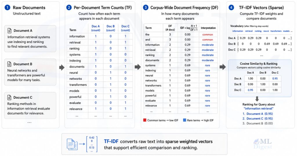
Before BM25, the dominant approach was TF-IDF (Term Frequency-Inverse Document Frequency). The idea is simple: a word is important in a document if it appears often (high TF) but is rare across all documents (high IDF). The combined score ranks documents by relevance.
But TF-IDF has two notable weaknesses:
- Unbounded term frequency: A document that mentions “cat” 100 times scores 10x higher than one that mentions it 10 times. But is a document with 100 mentions really 10x more relevant? At some point, more mentions stop adding meaningful signal.
- No document length normalization: A 10,000-word document will naturally contain more occurrences of any term than a 100-word summary, even if the summary is far more on-topic.
1.2 The Birth of BM25
BM25, which stands for Best Match 25, emerged from a series of probabilistic retrieval experiments conducted through the Text REtrieval Conference evaluations in the 1990s. The “25” refers to the 25th iteration in that research series.
BM25 introduced two elegant solutions: term frequency saturation and document length normalization, both controlled by tunable parameters.
2. The Intuition Behind BM25
Before looking at any equations, consider two core ideas:
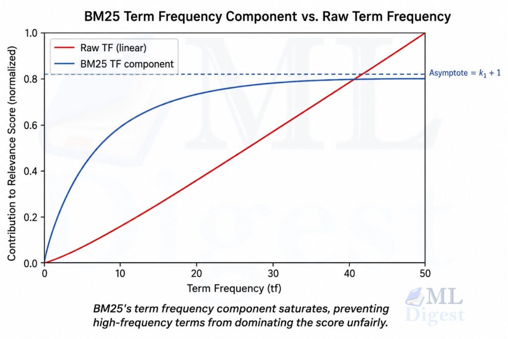
Idea 1: Diminishing returns on term frequency. The first mention of “neural network” in a document gives you a lot of information. The 50th mention gives you almost nothing new. BM25 models this with a saturation curve: relevance grows quickly with the first few term occurrences and then levels off.
Idea 2: Length normalization. A 5,000-word document mentioning “transformer” 20 times is less focused than a 500-word document mentioning it 20 times. BM25 penalizes longer documents relative to the average document length in your corpus.
3. The BM25 Formula
Given a query $Q$ containing terms $q_1, q_2, \ldots, q_n$ and a document $D$, the BM25 score is:
$$\text{BM25}(D, Q) = \sum_{i=1}^{n} \text{IDF}(q_i) \cdot \frac{f_{q_i,D} \cdot (k_1 + 1)}{f_{q_i,D} + k_1 \cdot \left(1 – b + b \cdot \dfrac{|D|}{\text{avgdl}}\right)}$$
Each term in this sum measures how much query term $q_i$ contributes to the relevance of document $D$. Let us walk through each piece.
3.1 The IDF Component
$$\text{IDF}(q_i) = \ln\left(\frac{N – n_{q_i} + 0.5}{n_{q_i} + 0.5} + 1\right)$$
Where:
- $N$ is the total number of documents in the corpus
- $n_{q_i}$ is the number of documents containing term $q_i$
- The $+0.5$ smoothing term prevents division by zero and stabilizes scores for very common or very rare terms
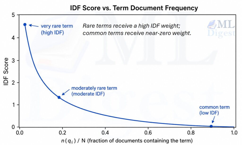
If a term appears in almost every document (like “the”), IDF approaches zero, and the term barely influences ranking. If a term appears in only a few documents, IDF is large, making matches on that term highly discriminative.
3.2 The TF Saturation Component
$$\text{TF_sat}(q_i, D) = \frac{f_{q_i,D} \cdot (k_1 + 1)}{f_{q_i,D} + k_1 \cdot \left(1 – b + b \cdot \dfrac{|D|}{\text{avgdl}}\right)}$$
where $f_{q_i,D}$ is the raw term frequency of $q_i$ in document $D$. $\text{avgdl}$ is the average document length in the corpus.
The numerator $f_{q_i,D} \cdot (k_1 + 1)$ scales with raw term frequency, where $k_1 + 1$ is the maximum possible contribution from term frequency.
The denominator grows with term frequency but also includes a length normalization factor. This creates a saturation effect: the first few occurrences move the score a lot, and additional repeats contribute progressively less. As $f_{q_i,D} \to \infty$, the ratio approaches $(k_1 + 1)$, so no single term can grow without bound.
3.3 The Parameters $k_1$ and $b$
These two parameters give BM25 its flexibility:
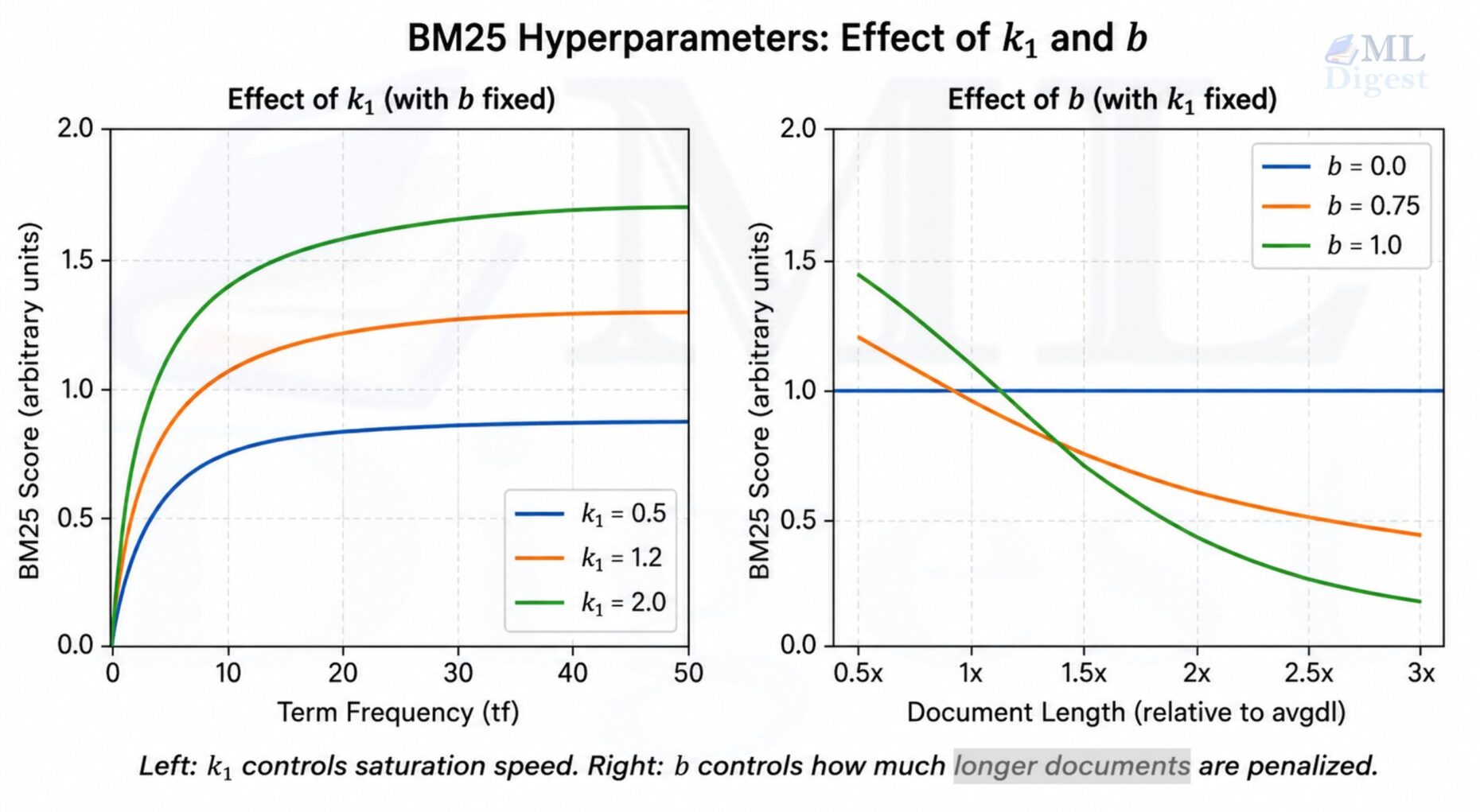
$k_1$ (term frequency saturation): Controls how quickly the TF component saturates.
- A higher $k_1$ means raw term frequency matters more (slower saturation).
- A lower $k_1$ (toward 0) approaches binary matching: the term is present or not.
- Typical values: $k_1 \in [1.2, 2.0]$.
$b$ (document length normalization): Controls how much document length affects the score.
- $b = 1.0$: Full normalization, longer documents are penalized maximally.
- $b = 0.0$: No normalization, document length is ignored.
- Typical value: $b = 0.75$.
The denominator’s length normalization term $\left(1 – b + b \cdot \dfrac{|D|}{\text{avgdl}}\right)$ is worth examining closely. When $|D| = \text{avgdl}$ (the document is average length), this equals $1 – b + b = 1$, meaning no adjustment. Longer documents get a denominator greater than 1, reducing the score. Shorter documents get a denominator less than 1, boosting the score.
4. BM25 vs. TF-IDF: A Side-by-Side Comparison
| Property | TF-IDF | BM25 |
|---|---|---|
| Term frequency handling | Linear, unbounded | Saturating, bounded by $k_1 + 1$ |
| Length normalization | Optional, simple | Built-in, tunable with $b$ |
| IDF smoothing | Varies by implementation | Robust Robertson IDF with $+0.5$ smoothing |
| Empirical performance | Reasonable baseline | Consistently stronger on TREC benchmarks |
| Parameters | None (or minimal) | $k_1$, $b$ (well-studied defaults exist) |
5. Implementing BM25 from Scratch
The best way to solidify understanding is to implement BM25 yourself. Below is a clean, self-contained implementation using only Python and NumPy.
import numpy as np
from collections import Counter
import math

class BM25:
    """
    A minimal BM25 implementation.

    Parameters
    ----------
    k1 : float
        Term frequency saturation parameter. Higher values give more
        weight to term frequency. Typical range: 1.2 to 2.0.
    b : float
        Document length normalization parameter. 0.0 = no normalization,
        1.0 = full normalization. Typical value: 0.75.
    """

    def __init__(self, k1: float = 1.5, b: float = 0.75):
        self.k1 = k1
        self.b = b
        self.corpus_size = 0
        self.avgdl = 0.0
        self.doc_freqs = []        # term frequencies per document
        self.idf = {}              # IDF scores per term
        self.doc_lengths = []      # number of tokens per document

    def fit(self, corpus: list[list[str]]) -> "BM25":
        """
        Build the index from a tokenized corpus.

        Parameters
        ----------
        corpus : list of list of str
            Each inner list is a tokenized document.
        """
        self.corpus_size = len(corpus)
        self.doc_lengths = [len(doc) for doc in corpus]
        self.avgdl = sum(self.doc_lengths) / self.corpus_size

        # Count term frequencies per document
        self.doc_freqs = [Counter(doc) for doc in corpus]

        # Count how many documents each term appears in
        df = Counter()
        for freq_map in self.doc_freqs:
            for term in freq_map:
                df[term] += 1

        # Robertson IDF formula with +0.5 smoothing
        for term, doc_count in df.items():
            numerator = self.corpus_size - doc_count + 0.5
            denominator = doc_count + 0.5
            self.idf[term] = math.log(numerator / denominator + 1)

        return self

    def score(self, query: list[str], doc_index: int) -> float:
        """Compute BM25 score for a single document given a query."""
        score = 0.0
        doc_freq = self.doc_freqs[doc_index]
        dl = self.doc_lengths[doc_index]

        # Length normalization factor
        length_norm = 1 - self.b + self.b * (dl / self.avgdl)

        for term in query:
            if term not in self.idf:
                continue  # term not in corpus, contributes 0

            tf = doc_freq.get(term, 0)
            idf = self.idf[term]

            # BM25 TF component with saturation
            tf_score = (tf * (self.k1 + 1)) / (tf + self.k1 * length_norm)

            score += idf * tf_score

        return score

    def get_scores(self, query: list[str]) -> np.ndarray:
        """Return BM25 scores for all documents in the corpus."""
        return np.array([self.score(query, i) for i in range(self.corpus_size)])

    def get_top_n(self, query: list[str], documents: list, n: int = 5) -> list:
        """Return the top-n most relevant documents for a query."""
        scores = self.get_scores(query)
        top_indices = np.argsort(scores)[::-1][:n]
return [(documents[i], scores[i]) for i in top_indices]Now, let us see it in action:
# A tiny corpus of sentences (pre-tokenized)
corpus = [
    "the quick brown fox jumps over the lazy dog".split(),
    "machine learning models learn from data".split(),
    "neural networks are a type of machine learning model".split(),
    "bm25 is a ranking function used in information retrieval".split(),
    "information retrieval systems rank documents by relevance".split(),
    "deep learning is a subset of machine learning".split(),
]

# Original documents (strings) for display
documents = [
    "The quick brown fox jumps over the lazy dog.",
    "Machine learning models learn from data.",
    "Neural networks are a type of machine learning model.",
    "BM25 is a ranking function used in information retrieval.",
    "Information retrieval systems rank documents by relevance.",
    "Deep learning is a subset of machine learning.",
]

# Build BM25 index
bm25 = BM25(k1=1.5, b=0.75)
bm25.fit(corpus)

# Query
query = "machine learning retrieval".split()
results = bm25.get_top_n(query, documents, n=3)

print("Top results for query:", " ".join(query))
print("-" * 50)
for doc, score in results:
print(f"Score: {score:.4f} | {doc}")Expected output:
Top results for query: machine learning retrieval
--------------------------------------------------
Score: 1.6834 | Deep learning is a subset of machine learning.
Score: 1.5620 | Machine learning models learn from data.
Score: 1.3125 | Neural networks are a type of machine learning model.
This toy implementation computes a score for every document, which is perfect for learning but not how production retrieval systems scale. Real search engines use an inverted index: for each term, they store a posting list of documents containing that term along with term frequencies, so query evaluation only touches documents that share at least one token with the query.
6. BM25 in the Modern ML Stack
Even as neural retrieval methods like Dense Passage Retrieval (DPR) and ColBERT have gained traction, BM25 remains highly relevant for several reasons.
6.1 BM25 in popular libraries
The rank_bm25 library is the most widely used Python library for BM25.
# Using rank_bm25 (pip install rank-bm25)
from rank_bm25 import BM25Okapi

documents = [
    "The quick brown fox jumps over the lazy dog.",
    "Machine learning models learn from data.",
    "Neural networks are a type of machine learning model.",
    "BM25 is a ranking function used in information retrieval.",
    "Information retrieval systems rank documents by relevance.",
    "Deep learning is a subset of machine learning.",
]

tokenized_corpus = [doc.lower().split() for doc in documents]
bm25 = BM25Okapi(tokenized_corpus)

query = "machine learning retrieval".lower().split()
scores = bm25.get_scores(query)

for doc, score in zip(documents, scores):
print(f"{score:.4f} {doc}")However, bm25s is a newer library focused on very fast sparse lexical retrieval in Python using NumPy, sparse matrices, and optional Numba acceleration. It also supports several BM25 variants such as BM25+.
# Using bm25s (pip install bm25s)
import bm25s

corpus = [doc.lower() for doc in documents]
corpus_tokens = bm25s.tokenize(corpus)

retriever = bm25s.BM25(k1=1.5, b=0.75)
retriever.index(corpus_tokens)

query_tokens = bm25s.tokenize("machine learning retrieval")
results, scores = retriever.retrieve(query_tokens, corpus=documents, k=3)

for doc, score in zip(results[0], scores[0]):
print(f"{score:.4f} {doc}")LlamaIndex and LangChain both offer native BM25 retriever integrations.
6.2 Hybrid Search
Modern search systems often combine BM25 with dense vector search in a pattern called hybrid retrieval:
- BM25 retrieves a candidate set of documents based on exact keyword overlap.
- A dense encoder (e.g., a fine-tuned sentence transformer) re-ranks the candidates using semantic similarity.
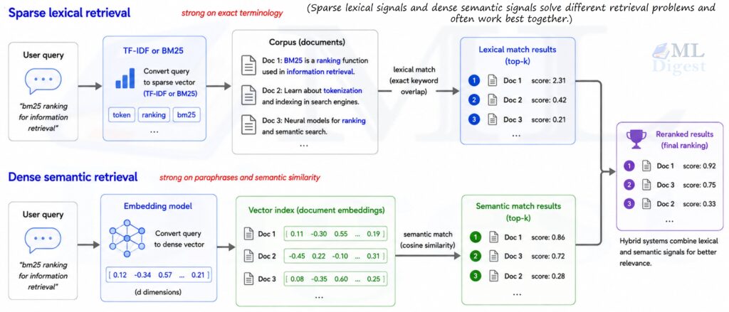
This hybrid approach exploits BM25’s strength (exact term matching, zero inference cost) and dense retrieval’s strength (semantic understanding). Tools like Elasticsearch’s hybrid search and Weaviate’s BM25 + vector fusion implement this pattern.
The dense side of that stack depends on learned vector representations from an embedding layer, which is why it can recover semantically related passages even when the exact query terms do not appear verbatim.
6.3 BM25 in RAG Pipelines
In Retrieval-Augmented Generation, BM25 serves as an efficient first-stage retriever. The pipeline looks like this:
Query → BM25 retrieval (top-k) → Re-ranker or LLM → Generated answerBM25 is well-suited for this role because it requires no GPU at query time, relies on inverted index lookups that scale to millions of documents, and handles rare or technical terms (product codes, proper nouns, domain jargon) that dense encoders may not generalize well to. A typical configuration retrieves between 50 and 200 candidates with BM25 before a cross-encoder or generative model processes the final top-k. In practice, many RAG systems index chunks rather than full documents so BM25 can retrieve focused passages instead of entire long files.
6.4 Using BM25 in Elasticsearch
In production, you would rarely implement BM25 yourself. Elasticsearch uses BM25 by default (since version 5.0). Here is how you configure the parameters directly in a mapping:
{
  "settings": {
    "similarity": {
      "custom_bm25": {
        "type": "BM25",
        "k1": 1.5,
        "b": 0.75
      }
    }
  },
  "mappings": {
    "properties": {
      "content": {
        "type": "text",
        "similarity": "custom_bm25"
      }
    }
  }
}7. Practical Tips and Best Practices
7.1 Preprocessing Matters
BM25 is a bag-of-words model; the quality of your tokenization has a large effect on results.
Modern neural systems often soften vocabulary fragmentation with subword tokenizers such as Byte Pair Encoding (BPE), but BM25 still depends directly on whatever final tokens you choose to index.
Index-time and query-time preprocessing must match. If documents are lowercased but queries are not, or punctuation is stripped only on one side, retrieval quality drops silently because exact token overlap is broken.
Standard preprocessing steps include:
- Lowercasing: “Neural” and “neural” should be the same token.
- Stop word removal: Common words like “the,” “is,” and “a” carry little discriminative signal.
- Stemming or lemmatization: “run,” “runs,” and “running” should ideally map to the same root. Libraries like NLTK and spaCy cover these steps.
Stop word handling is also domain-dependent. In legal, medical, or product-search corpora, seemingly common words may still carry useful signal, so it can be better to keep them indexed and let IDF downweight them rather than removing them aggressively.
import nltk
from nltk.corpus import stopwords
from nltk.stem import PorterStemmer

nltk.download("stopwords", quiet=True)
stop_words = set(stopwords.words("english"))
stemmer = PorterStemmer()

def preprocess(text: str) -> list[str]:
    tokens = text.lower().split()
    tokens = [t for t in tokens if t.isalpha() and t not in stop_words]
    tokens = [stemmer.stem(t) for t in tokens]
return tokens7.2 Tuning $k_1$ and $b$
The defaults ($k_1 = 1.5$, $b = 0.75$) work well across many domains, but it is worth tuning them on your specific data if you have labeled relevance judgments. Key intuitions:
- Short, precise documents (e.g., product titles): Use a lower $b$ (0.3 to 0.5) since length normalization is less meaningful.
- Long documents (e.g., legal or academic text): Use a higher $b$ (0.75 to 1.0) to correct for verbosity.
- Keyword-heavy queries: A higher $k_1$ rewards documents that repeat the term many times.
7.3 Handling Out-of-Vocabulary Terms
If a query term does not appear in any indexed document, its IDF score is zero and it contributes nothing to the ranking. This is expected behavior, but it means BM25 cannot bridge out-of-vocabulary words on its own. Neural approaches often reduce that pain with subword-aware representations such as FastText or tokenizers like BPE, but BM25 itself still needs literal token overlap. If your queries often use synonyms or paraphrases not present in the corpus, combine BM25 with a semantic retrieval layer.
7.4 When BM25 Struggles
BM25 works best when:
- The query and documents share vocabulary (no paraphrase mismatch).
- Term presence is a reliable signal of relevance.
It struggles when:
- Relevance depends on semantics, context, or user intent not expressible in keywords.
- Queries are very short (1-2 words), where IDF weighting has little to differentiate candidates.
- Documents are extremely short (e.g., tweets), where length normalization has minimal effect.
8. BM25 Variants
The BM25 formula has spawned several variants worth knowing:
- BM25+ (Lv and Zhai, 2011): Addresses a lower-bounding issue in standard BM25’s length normalization, which can unfairly suppress scores for long matching documents. BM25+ adds a small constant $\delta$ to the TF component.
$$\text{TF_sat}^{+} = \delta + \frac{f_{q_i,D} \cdot (k_1 + 1)}{f_{q_i,D} + k_1 \cdot \text{length_norm}}$$ - BM25F (Robertson et al., 2004): Extends BM25 to structured documents with multiple fields (title, body, anchor text), each with its own weight and length normalization. Elasticsearch’s
combined_fieldsquery uses a BM25F-style scoring approximation, but Elasticsearch does not generally replace standard per-field BM25 scoring with BM25F everywhere. - BM25-Adpt (Trotman et al., 2014): Adapts $k_1$ dynamically per query term based on corpus statistics, removing the need for manual tuning.
Summary
BM25 is a beautifully engineered ranking function that has stood the test of time. Here are the key takeaways:
- It improves on TF-IDF by adding term frequency saturation (controlled by $k_1$) and document length normalization (controlled by $b$).
- The Robertson IDF weighting ensures that rare, discriminative terms drive the ranking.
- Default parameters ($k_1 = 1.5$, $b = 0.75$) generalize well, but tuning on domain-specific data can improve performance.
- In modern ML systems, BM25 is most powerful as the first stage in a hybrid retrieval pipeline, paired with dense vector search.
- Preprocessing (tokenization, stop word removal, stemming) has a large practical impact on BM25 performance.

Silpa brings 5 years of experience in working on diverse ML projects, specializing in designing end-to-end ML systems tailored for real-time applications. Her background in statistics (Bachelor of Technology) provides a strong foundation for her work in the field. Silpa is also the driving force behind the development of the content you find on this site.

Happy is a seasoned ML professional with over 15 years of experience. His expertise spans various domains, including Computer Vision, Natural Language Processing (NLP), and Time Series analysis. He holds a PhD in Machine Learning from IIT Kharagpur and has furthered his research with postdoctoral experience at INRIA-Sophia Antipolis, France. Happy has a proven track record of delivering impactful ML solutions to clients.
Subscribe to our newsletter!