Architecture of the Embedding Layer During Training of LLMs

The embedding layer in an LLM is a critical component that maps discrete input tokens (words, subwords, or characters) into continuous vector representations that the model can process. These dense vectors exist in a high-dimensional space and encode semantic and syntactic information, enabling the model to capture contextual and relational patterns in language.

This article covers the architecture of embedding layers, how token and positional embeddings work together to form the input representation, and how these parameters are learned during training.

Architecture of the Embedding Layer

The embedding layer is essentially a lookup table implemented as a matrix. It has three main components: token embeddings, positional embeddings, and the combined input representation.

Token Embedding: Capturing Semantic Meaning

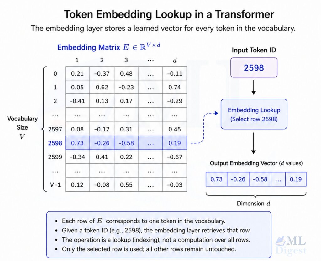
• Embedding Matrix Dimensions: $V \times d$, where:
• $V$ = Vocabulary size (number of unique tokens)
• $d$ = Embedding dimension (a model hyperparameter, e.g., 768 for BERT, 12288 for GPT-3)
• Each row in the matrix corresponds to a vector representation of a token in the vocabulary.
• Given an input token index $i$, the embedding layer retrieves the $i$-th row of the embedding matrix as that token’s vector.

Positional Embedding

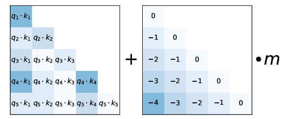
Transformer self-attention is permutation-equivariant, meaning it produces the same output regardless of input order. Positional embeddings break this symmetry by injecting information about where each token sits in the sequence.

• Positional embeddings are typically added to (and sometimes concatenated with) token embeddings.
• They can be learned or fixed:
• Learned: A trainable matrix of shape $L \times d$, where $L$ is the maximum sequence length.
• Fixed (sinusoidal): Computed algorithmically using sine and cosine functions at different frequencies, as introduced in the original Transformer paper (Vaswani et al., 2017).

Modern Positional Encoding Methods

Recent LLMs have moved beyond absolute positional embeddings in favor of methods that encode relative position directly into the attention computation:

• Rotary Position Embedding (RoPE): Encodes absolute position via a rotation matrix applied to query and key vectors, while naturally incorporating relative position information into the attention score. Used in LLaMA, PaLM, and many open-source LLMs.
• ALiBi (Attention with Linear Biases): Instead of adding positional embeddings to token vectors, ALiBi applies a linear bias to attention scores proportional to the distance between tokens. This enables strong length extrapolation (training on short sequences but inferring on longer ones).

Input Representation

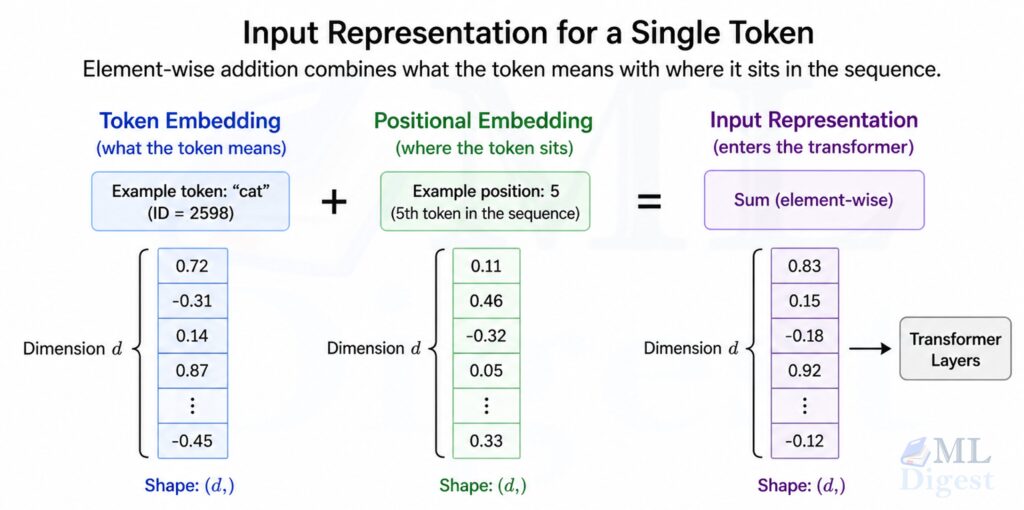
Token and positional embeddings are combined element-wise via addition to form the final input for the transformer stack. Addition is preferred over concatenation because it preserves the embedding dimension, keeping the model’s parameter count and computation cost constant regardless of how positional information is encoded. For each token at position $p$ in a sequence:

$$
\text{Input Representation} = \text{Token Embedding} + \text{Positional Embedding}(p)
$$

This combined representation captures both the semantic meaning and the sequential order of the input, allowing the model to distinguish between identical tokens appearing at different positions.

How Embedding Parameters Are Learned

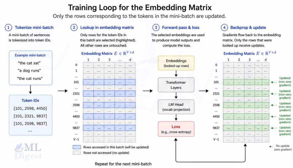
The parameters of the embedding matrix are learned during training through the same backpropagation mechanism that updates all other model weights. The process follows the standard forward-backward loop:

Forward Pass

1. Input Tokenization: Text is tokenized into token IDs. Common tokenization strategies for LLMs include:

• Subword-level: Uses subword units via algorithms like Byte Pair Encoding (BPE) or WordPiece. This is the dominant approach in modern LLMs.
• Word-level: Splits input into whole words (rarely used for LLMs due to large vocabulary sizes).
• Character-level: Splits into individual characters (less common for LLMs).

Note: The embedding matrix can optionally be initialized with pre-trained vectors from methods like Word2Vec, GloVe, or FastText, though most modern LLMs learn embeddings from scratch.

2. Embedding Lookup: Each token ID is mapped to its corresponding row in the embedding matrix. Positional embeddings are retrieved (if learned) or computed (if fixed) for each position.
3. Vector Representation: The final embedding for each token is formed by adding the token embedding and the positional embedding.
4. Processing by Transformer Layers: These embeddings are fed into subsequent layers (self-attention, feedforward networks) to compute predictions.

Backward Pass

1. Loss Computation: The model compares predictions to ground truth and computes a loss (e.g., cross-entropy for language modeling).
2. Gradient Computation: Gradients are computed for all model parameters, including the embedding matrix, with respect to the loss.
3. Parameter Updates: Gradients are used to update the embedding matrix via optimization techniques such as Adam.

An important property of this process: if the $i$-th token appears in a training batch, only the corresponding row of the embedding matrix receives a gradient update in that step. Rows for tokens not present in the batch remain unchanged. As a practical consequence, rare tokens accumulate far fewer gradient updates over training and often end up with lower-quality embeddings than high-frequency tokens. This is one reason subword tokenization strategies such as BPE are preferred: they decompose rare words into frequent subword units, ensuring that even uncommon vocabulary receives adequate training signal. See How LLMs Handle Out-of-Vocabulary Words for a closer look at how modern models address vocabulary limitations.

Walkthrough Example

Consider training a transformer-based LLM on the sentence "The cat sat.".

Step 1: Tokenization

Sentence: "The cat sat."
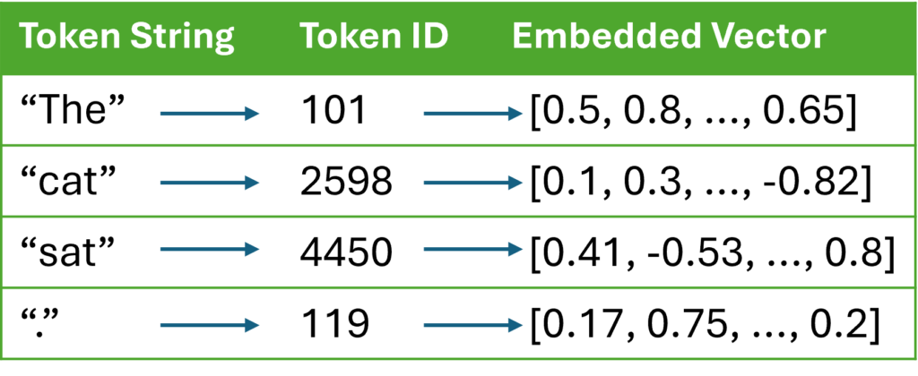
Tokens: ["The", "cat", "sat", "."]
Token IDs: [101, 2598, 4450, 119]

Step 2: Token Embedding Lookup

Retrieve embeddings for each token ID from the embedding matrix ($V \times d$):

Embedding(101)  = [0.5, 0.8, ...]
Embedding(2598) = [0.1, 0.3, ...]

Step 3: Positional Embedding

Retrieve or compute positional vectors:
$\text{Position}(0) = [0.01, 0.02, …]$, $\text{Position}(1) = [-0.03, 0.05, …]$

Step 4: Summation

Input Vector 0 = Embedding(101)  + Position(0)
Input Vector 1 = Embedding(2598) + Position(1)

These combined vectors are then passed to the first transformer layer.

Techniques for Learning Better Embeddings

1. Pre-training objectives:
   Embeddings are shaped by the model’s pre-training objective:

• Masked language modeling (e.g., BERT): Predicting masked tokens forces embeddings to encode bidirectional context.
• Causal language modeling (e.g., GPT): Predicting the next token encourages embeddings to capture sequential dependencies.

1. Regularization:

• Regularization techniques like dropout or weight decay are applied to embedding layers to prevent overfitting.
• Subword tokenization (BPE, WordPiece) keeps the vocabulary size manageable, reducing the number of embedding parameters while maintaining coverage of rare words.

1. Weight tying:
   Many LLMs tie the input embedding matrix with the output projection layer (the matrix that maps hidden states back to vocabulary logits). This technique, explored in detail in Weight Tying in Transformers, reduces parameter count and improves performance, especially for smaller models. The intuition is that a token’s input representation and its output representation should occupy a similar region in the vector space, so sharing the same matrix enforces this consistency directly.

Properties and Benefits of Embeddings

Semantic structure: Trained embeddings capture meaningful relationships between tokens. A classic demonstration is word analogy arithmetic:
$$
\text{vec(“king”)} – \text{vec(“man”)} + \text{vec(“woman”)} \approx \text{vec(“queen”)}
$$

Compact representation: The embedding layer converts sparse, one-hot-like token IDs into dense vectors that carry far more information per dimension.

Transfer and generalization: Embeddings learned during pre-training on large corpora generalize well to downstream tasks, which is one reason LLMs exhibit strong zero-shot and few-shot performance.

Positional awareness: Positional embeddings allow transformers to distinguish token order, which is essential since the self-attention mechanism itself is order-agnostic. Fixed (sinusoidal) encodings can generalize to sequence lengths not seen during training, while learned encodings tend to perform better within the trained length range.

Summary

The embedding layer is a parameterized lookup table learned via backpropagation during model training. Token embeddings capture the semantic properties of language through pre-training, while positional embeddings (whether sinusoidal, learned, or relative methods such as RoPE and ALiBi) provide the sequential context that transformers need. Design choices such as weight tying and subword tokenization further shape the quality and efficiency of these representations. Together, these components form the foundation on which all subsequent transformer computation builds.