Imagine you hire a brilliant consultant who spent years studying everything published up to the day they joined your company. On day one, they are extraordinarily sharp. But as months pass, the industry shifts, your codebase evolves, your customers change their behavior, and new research overturns old assumptions. Your consultant, however, has stopped reading. They still answer confidently, but the gap between what they know and what the world looks like is quietly widening. Eventually, the advice they give starts to feel stale, occasionally wrong, and sometimes dangerously overconfident.
Large Language Models are that consultant. They are trained on a snapshot of the world, deployed into a world that never stops moving, and then asked to perform at the same level indefinitely. The result is what practitioners call LLM performance degradation: a gradual or sudden decline in the quality, relevance, and reliability of a model’s outputs.
This article walks through every major reason an LLM can degrade, gives you the conceptual and mathematical tools to understand what is happening under the hood, and then equips you with practical, code-backed strategies to fix it.
1. What “Performance Degradation” Actually Means
Before diagnosing causes, it helps to be precise about what degradation looks like in practice. It is not one thing. It is a family of failure modes that can appear at different times, for different reasons, and at different severity levels.
Here are the main manifestations you will encounter:
- Accuracy drop on known benchmarks. The model answers factual questions it once got right incorrectly, or its MMLU / HumanEval scores fall after fine-tuning.
- Hallucination increase. The model begins confabulating facts, citations, or code that look plausible but are wrong.
- Distribution mismatch errors. The model struggles with new terminology, new APIs, or new domain-specific patterns that did not exist in its training data.
- Refusal drift. After alignment fine-tuning, the model over-refuses benign requests or produces overly cautious, low-utility responses.
- Instruction-following regression. A model that once reliably followed structured output formats or multi-step instructions begins producing malformed responses.
Each of these has a different root cause, and, importantly, a different fix. Let us work through them one by one.
2. The Root Causes
2.1 Distribution Shift: The World Moved, the Model Did Not
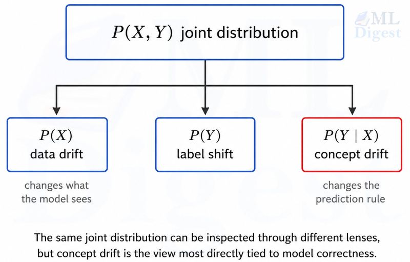
The single most common cause of degradation is distribution shift: the statistical properties of the inputs the model sees at deployment time differ from those it saw during training.
Formally, let $P_{\text{train}}(x)$ be the distribution of inputs during training and $P_{\text{deploy}}(x)$ be the distribution at inference time. Degradation happens when:
$$P_{\text{train}}(x) \neq P_{\text{deploy}}(x)$$
This gap takes several forms:
Data drift is the most common: the input distribution changes but the underlying mapping from input to correct output remains the same. A model trained on formal English news articles will underperform on casual social media text even if the task (sentiment classification, say) is unchanged.
Label shift is subtler: the prior probability of the output classes changes. If a fraud-detection LLM was trained when fraudulent transactions made up 2% of traffic and fraud now accounts for 15%, the model’s calibrated confidence scores are systemically wrong.
Concept drift is the most insidious: the relationship between input and correct output itself changes. A code assistant trained before a framework’s major version change will confidently suggest deprecated APIs.
2.2 Temporal Knowledge Decay
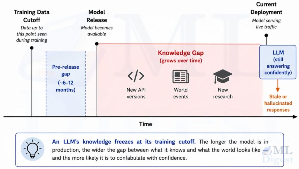
Every LLM has a knowledge cutoff: a date after which its training data contains little or nothing. Early GPT-4 deployments, for example, were trained on data with a September 2021 cutoff, and many 2024-era open models were trained on corpora collected before 2024. The world does not pause for training runs.
The practical consequence is that a model asked about events, people, companies, libraries, or regulations that emerged after its cutoff will either hallucinate an answer or correctly flag its ignorance. Over time, this gap compounds. A model deployed for two years after its cutoff is essentially a time traveler trying to give advice in a world they have never seen.
What makes this particularly tricky is that the model does not know what it does not know. It can confidently describe the API of torch.nn.functional as it existed in 2022, having no awareness that it changed in 2024. The failure mode is silent.
2.3 Catastrophic Forgetting During Fine-Tuning
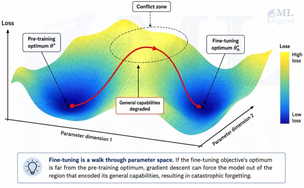
When you fine-tune a pre-trained LLM on a new, narrow dataset, you are adjusting the same weights that encode its general world knowledge. The optimizer dutifully pushes those weights toward the fine-tuning objective, which can overwrite previously stored representations.
This phenomenon is known as catastrophic forgetting. The core tension is captured by the loss landscape. During pre-training, the model found a set of parameters $\theta^*$ that minimized the general language modeling loss $\mathcal{L}_{\text{pre}}(\theta)$. Fine-tuning minimizes a new task-specific loss $\mathcal{L}_{\text{ft}}(\theta)$. The optimal $\theta$ for each objective may be in very different regions of parameter space:
$$\theta_{\text{ft}}^* = \arg\min_\theta \mathcal{L}_{\text{ft}}(\theta) \quad \text{while} \quad \mathcal{L}_{\text{pre}}(\theta_{\text{ft}}^*) \gg \mathcal{L}_{\text{pre}}(\theta^*)$$
In plain terms: the fine-tuned model has gotten better at the new task but has “forgotten” how to do general reasoning, follow instructions, or write coherent prose.
2.4 The Lost-in-the-Middle Effect and Context Window Limits
Modern LLMs have context windows ranging from 8K to over 1M tokens. You might assume that a bigger context window means better performance at long contexts. In practice, the relationship is not that simple.
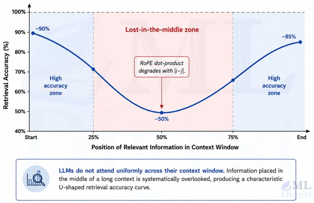
Liu et al. (2023) demonstrated the lost-in-the-middle phenomenon: LLMs reliably use information placed at the very beginning and very end of a long context, but significantly underutilize information buried in the middle. This means that as you push more content into the context window, the model’s effective ability to ground its responses in that content degrades non-linearly.
One common intuition is that long-range interactions become harder to preserve as token distance grows — a consequence of how the attention mechanism computes pairwise relevance scores across all token positions. In RoPE-style models, positional information is folded into the attention score for a token at position $i$ attending to a key at position $j$:
$$\text{Attn}(i, j) \propto \exp\left(\frac{q_i \cdot k_j^{\text{RoPE}}}{\sqrt{d_k}}\right)$$
RoPE does encode a distance-sensitive bias, and the original RoPE paper notes decaying inter-token dependency with increasing relative distance. Unlike absolute position embeddings that assign a fixed positional vector to each index regardless of context, RoPE and other relative schemes embed distance directly into the attention computation, which is part of why long-range interactions weaken as token distance grows. But the lost-in-the-middle result is empirical: it reflects a combination of architecture, training, and prompt layout, not RoPE alone.
2.5 Quantization-Induced Degradation
Storing the weights of a 70B parameter model in full float32 precision requires roughly 280 GB of memory before accounting for KV cache and other runtime overheads, which is prohibitively expensive. Quantization compresses weights to lower bit-widths (INT8, INT4, even INT2) to make deployment practical.
The price is precision loss. When a weight $w$ is quantized from float32 to an integer representation, the quantized value $\hat{w}$ and the resulting quantization error $\epsilon_q$ are:
$$\hat{w} = \text{round}\left(\frac{w}{s}\right) \cdot s, \qquad \epsilon_q = w \;-\; \hat{w}$$
where $s$ is the quantization scale factor. This error accumulates across layers. For most tasks, well-implemented 8-bit and even 4-bit quantization causes minimal perplexity increase. But edge cases matter: mathematical reasoning, precise code generation, and calibrated confidence often degrade noticeably at INT4 and below.
The layers most sensitive to quantization are the attention projection matrices and feed-forward weights, where a small number of channels carry disproportionately large activation magnitudes. Crushing those outlier values to low-bit representations produces the largest perplexity spikes.
2.6 The Alignment Tax: Over-Refusal and Helpfulness Regression
RLHF (Reinforcement Learning from Human Feedback) and DPO (Direct Preference Optimization) have made modern LLMs dramatically safer and more pleasant to use. But alignment fine-tuning imposes a cost that is easy to overlook: the model can become over-cautious.
When a reward model trained on human preferences assigns low reward to anything that looks potentially harmful, and that signal is used to update the base model, the model learns to refuse not just genuinely harmful prompts but also benign ones that superficially resemble them. This is the alignment tax: a reduction in raw capability and helpfulness that comes from safety optimization.
You can observe this as “sycophancy” (the model agrees with you even when you are wrong), “over-refusal” (the model declines clearly safe requests), or “hedging inflation” (every answer is padded with disclaimers that add no information). One way to contain some of these symptoms without retraining the model is to apply structured techniques to control the model’s output behavior, such as system prompt engineering and output format constraints, or to layer guardrails on top of the deployment: external classifiers and rule-based filters that intercept over-refusals or flag unsafe outputs before they reach the user.
3. Diagnosing Before You Fix
The right solution depends entirely on the right diagnosis. Before reaching for RAG or LoRA, you need to know which failure mode you are dealing with. Here is a practical diagnostic workflow.
Start by running your eval suite across a set of representative task categories and comparing each task’s current score against a baseline. A task is worth investigating if its score has dropped by more than about two percentage points in absolute terms — small fluctuations below that threshold are usually noise. For each task that has degraded, map it to its most likely root cause based on what that task actually exercises:
- Poor performance on questions about recent facts points to temporal knowledge decay.
- Regressions on static factual questions that the model previously answered correctly suggest catastrophic forgetting from a recent fine-tuning run.
- Failures on long-context retrieval tasks indicate the lost-in-the-middle effect.
- Drops in code generation quality can stem from distribution shift (new APIs, new frameworks) or quantization artifacts.
- Worse instruction-following scores often trace back to the alignment tax introduced by RLHF or DPO fine-tuning.
- Degraded mathematical reasoning is frequently caused by aggressive quantization or catastrophic forgetting.
Group all degraded tasks by their probable cause. To make this concrete: if recent factual QA drops from 0.82 to 0.61 and long-context retrieval drops from 0.74 to 0.58, while static QA and instruction-following hold roughly steady, the diagnosis points squarely at temporal knowledge decay and the lost-in-the-middle effect, leaving the fine-tuning and alignment axes in the clear.
For a broader measurement framework around capability, reliability, latency, and cost, pair this kind of triage with a dedicated LLM evaluation stack.
The key principle here is to decompose your eval suite by failure mode, not just by task category. A single “performance dropped on Q&A” diagnosis tells you nothing actionable. A diagnosis of “performance dropped specifically on Q&A about events after 2023” points directly at temporal knowledge decay and immediately suggests RAG as the fix.
4. Solutions
4.1 Retrieval-Augmented Generation (RAG) for Temporal Decay and Distribution Shift
If your model’s primary failure mode is temporal knowledge decay or distribution shift to new domain content, the most practical and widely-deployed solution is Retrieval-Augmented Generation (RAG), introduced by Lewis et al. at Facebook AI Research.
The core idea is elegantly simple: instead of trying to bake all world knowledge into model weights (a losing battle against time), you give the model a retrieval system — often combining sparse methods like BM25 with dense vector search — that fetches relevant, up-to-date documents at inference time and places them in the context window. The model’s job is then synthesis and reasoning, not memorization.
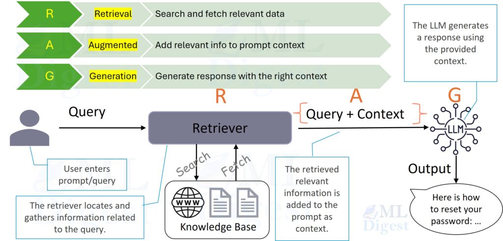
The key design decisions that separate good RAG systems from great ones:
- Chunking strategy matters. Fixed-size chunking is the easiest to implement but often splits sentences mid-thought. Semantic chunking (grouping by topic boundary) improves retrieval precision substantially.
- Reranking is worth the cost. A reranker applied to the top-20 retrieved chunks before selecting the top-3 can meaningfully improve final answer quality. Cross-encoders based on BERT are a common choice, and late-interaction retrievers such as ColBERT are also widely used in modern retrieval stacks.
- Citation grounding reduces hallucinations. Prompt the model to cite which context chunk supports each claim. This forces it to stay grounded and gives you an auditable trail.
If your corpus is rich in entities and relationships rather than standalone passages, knowledge-graph-based RAG can be a better fit than plain chunk retrieval.
4.2 Parameter-Efficient Fine-Tuning to Combat Catastrophic Forgetting
When you must fine-tune (for domain adaptation, instruction style, or task alignment), the most reliable way to preserve general capabilities is to change as few weights as possible. This is the insight behind LoRA (Low-Rank Adaptation), one of the most widely used parameter-efficient fine-tuning (PEFT) methods, introduced by Hu et al.
LoRA freezes the pre-trained weight matrix $W_0 \in \mathbb{R}^{d \times k}$ and learns only a low-rank perturbation:
$$W = W_0 + \Delta W = W_0 + BA$$
where $B \in \mathbb{R}^{d \times r}$ and $A \in \mathbb{R}^{r \times k}$ with rank $r \ll \min(d, k)$. Only $A$ and $B$ are updated during fine-tuning. The frozen $W_0$ is the “memory” of pre-training; the learned $BA$ is the “adapter” for the new task.
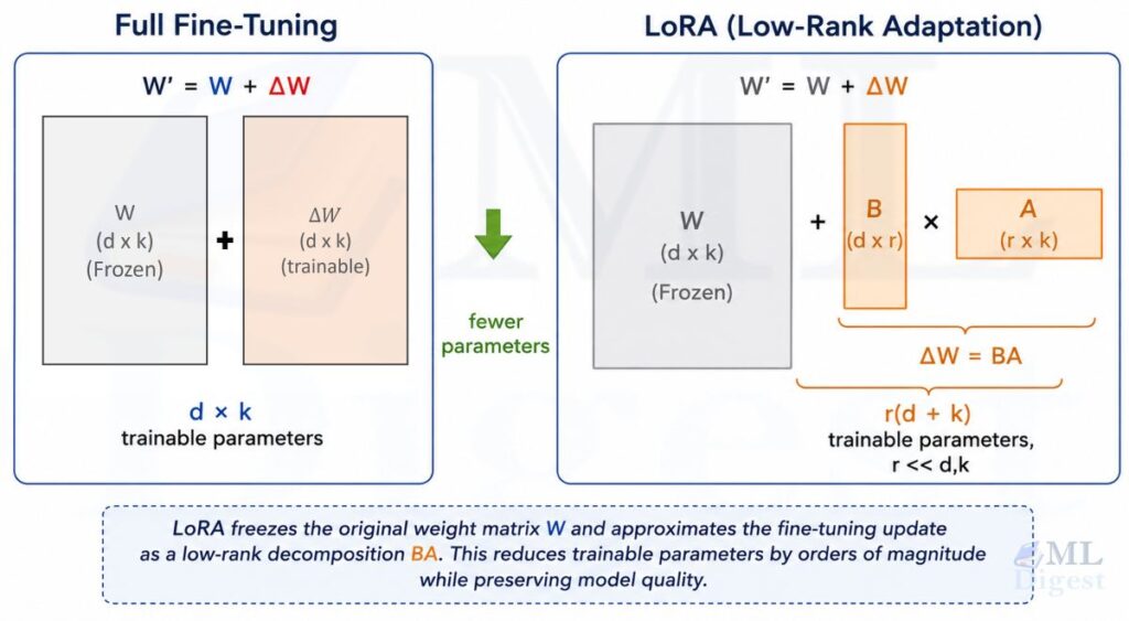
The parameter savings are dramatic. For a typical 7B model, full fine-tuning touches ~7 billion parameters. LoRA with $r = 16$ typically touches fewer than 30 million, roughly 0.4% of the original.
For memory-constrained environments, QLoRA (Quantized LoRA) by Dettmers et al. extends this further by quantizing the frozen base model weights to 4-bit NormalFloat (NF4) format while keeping the LoRA adapter in bfloat16, enabling fine-tuning of 65B parameter models on a single 48 GB GPU.
A practical tip: if you observe that fine-tuning is still causing forgetting despite LoRA, you can apply elastic weight consolidation (EWC) as a regularizer. EWC adds a penalty term to the loss that slows down updates to weights that were important for the pre-training objective:
$$\mathcal{L}_{\text{EWC}}(\theta) = \mathcal{L}_{\text{ft}}(\theta) + \frac{\lambda}{2} \sum_i F_i (\theta_i – \theta_i^*)^2$$
Here, $F_i$ is the Fisher information for parameter $i$ (an estimate of how important that parameter was for the pre-training task), $\theta_i^*$ are the pre-trained values, and $\lambda$ controls the regularization strength. The Fisher information effectively acts as a per-parameter learning rate damper: parameters that were crucial before change slowly.
4.3 Better Quantization: GPTQ and AWQ
Not all quantization is created equal. Naive round-to-nearest quantization treats all weights equally. Research has shown that LLM weights are not all equally important: a small number of outlier activations carry disproportionate amounts of information, and crushing them to INT4 causes severe perplexity spikes.
Two methods have emerged as practical standards for high-quality LLM quantization:
GPTQ (Frantar et al., 2022) frames quantization as a layer-wise reconstruction problem. For each linear layer, it finds the 4-bit weight matrix $\hat{W}$ that minimizes the output reconstruction error on a calibration set:
$$\hat{W} = \arg\min_{\hat{W}} | W X – \hat{W} X |_F^2$$
It solves this efficiently using second-order gradient information (the Hessian of the layer’s inputs), which allows it to quantize weights in an order that compensates for previously introduced errors.
AWQ (Activation-aware Weight Quantization) (Lin et al., 2023) takes a different approach: use activation statistics to identify a small fraction of salient weights or channels and rescale them so they survive low-bit weight-only quantization better. The key insight is that you can protect the most important signals without resorting to hardware-unfriendly mixed-precision handling for the whole layer.
A practical guideline: for production deployments where inference accuracy matters, prefer purpose-built LLM quantizers such as GPTQ or AWQ over generic post-training quantization flows. The calibration step takes minutes and the quality improvement is usually measurable.
If post-training compression still costs too much quality, quantization-aware training is the next lever to consider. For deployments where memory is the binding constraint, complementary compression techniques such as pruning and knowledge distillation offer different points on the efficiency-quality tradeoff curve and can be combined with quantization.
4.4 Addressing the Lost-in-the-Middle Problem
If your degradation traces back to long-context performance, you have several options, from the tactical to the architectural.
Tactically, restructure your prompts so that the most critical information appears at the beginning or end of the context window, not buried in the middle. This sounds obvious but is frequently overlooked in RAG pipelines that naively concatenate retrieved chunks in retrieval-score order.
Architecturally, consider whether you actually need a single massive context window or whether you can use a multi-hop retrieval strategy: retrieve, synthesize a compressed summary, then retrieve again based on the summary. This mirrors how humans read long documents and is often more robust than hoping the model attends uniformly to a 100K token context.
For evaluation, use the needle in a haystack: insert a specific fact (the “needle”) at varying depths in a long document (the “haystack”) and measure whether the model can retrieve it.
The mechanics are straightforward. Take a long filler document (several thousand words of neutral, repetitive text) and embed a single distinctive sentence (say, “the special magic number is 42”) at a controlled position: 10% of the way through, then 25%, 50%, 75%, and 90%. For each placement, send the full document to the model with a question that can only be answered by finding that sentence, and record whether the answer is correct. Repeat the sweep across several different total context lengths. The result is a depth-by-length grid of hit and miss outcomes, which you visualize as a heatmap. A healthy model shows near-uniform green across the grid. A model suffering from the lost-in-the-middle effect shows a band of red or orange in the middle-depth rows, brightening toward the top and bottom — the characteristic U-shaped retrieval curve.
4.5 Monitoring: Catching Degradation Before Your Users Do
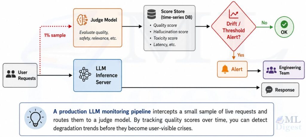
All the fixes above are reactive. The most professional approach to LLM performance management is continuous monitoring with automated alerting. The operational discipline is at the core of any mature MLOps practice so that degradation is caught the moment it begins rather than after it has affected thousands of users.
A minimal but effective monitoring stack has three components:
- A regression eval suite that runs on every model version change (new fine-tune, new quantized export, dependency update). This is your canary-in-the-coal-mine.
- Continuous production sampling where a random sample (say, 1%) of live inference requests is logged and scored by a separate judge model.
- Statistical drift detection on the input distribution, watching for sudden shifts in vocabulary, topic distribution, or query length that might signal that the user population or use case has changed.
For the third component, two metrics are particularly useful in practice. KL divergence measures how much the current input distribution $Q$ has shifted from the reference distribution $P$ established at training time.
A rising KL divergence over rolling windows is an early warning that the input space is drifting. Its limitation is that it is asymmetric and undefined when $Q(x) = 0$ for any $x$ that $P$ assigns nonzero probability. The Wasserstein distance (also called the “earth mover’s distance”) is more robust: it measures the minimum cost to transport the mass of one distribution to match the other, making it well-defined even when the distributions have non-overlapping support.
In practice, you apply these metrics not to raw token sequences but to a lower-dimensional embedding of each request (e.g., a sentence embedding), which makes the computation tractable.
4.6 Feedback Loops and Active Learning
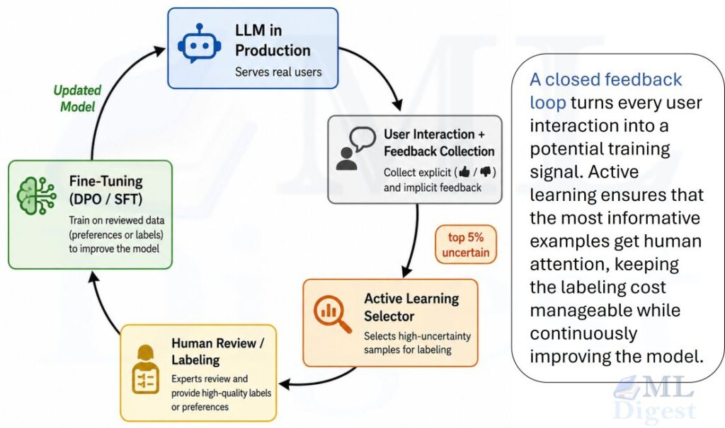
All the solutions so far treat the model as something you fix and redeploy. A more sustainable long-term approach is to build a continuous learning system that learns from its own mistakes, closing the loop between deployment and improvement.
The idea is straightforward: every interaction where a user corrects the model, rates a response poorly, or reformulates a question because the first answer was unsatisfactory is a training signal. Capturing and routing that signal back into the training pipeline is what separates a static deployed artifact from a living system.
User feedback integration is the first lever. Even a simple thumbs-up / thumbs-down widget generates a labeled dataset of good and bad responses over time. More structured feedback (e.g., “this code produced a runtime error” paired with the original prompt and the model’s answer) is even more valuable. This feedback can directly power a DPO fine-tuning run: the user-preferred response becomes the “chosen” example and the model’s original response becomes the “rejected” example.
Active learning takes a more targeted approach. Rather than labeling everything, you identify the requests where the model is least confident (high output entropy or low self-consistency across multiple samples) and prioritize those for human review. This dramatically reduces the labeling budget while concentrating effort on the examples that will teach the model the most.
One practical note: feedback loops can introduce their own degradation if not managed carefully. If you fine-tune exclusively on the prompts your current users ask, you risk distribution narrowing: the model becomes excellent at the current user population’s queries and worse at everything else. Periodically mixing in a broad general-purpose dataset alongside the feedback-driven fine-tuning data is the standard mitigation.
4.7 Safe Deployment: Versioning, A/B Testing, and Canary Rollouts
Even the best-tested model update can behave unexpectedly in production. The engineering discipline of safe deployment gives you a safety net: the ability to catch regressions early and roll back instantly. For a comprehensive view of hosting options and architectural tradeoffs that shape deployment risk, see the LLM deployment strategy guide.
Model versioning is the foundation. Every model artifact (weights, quantization config, tokenizer, adapter) should be tagged with a semantic version and stored in an artifact registry such as MLflow alongside its eval scores. This gives you a precise rollback target if a new version underperforms, rather than hunting through training run logs.
Canary deployments introduce a new model version to a small fraction of traffic (typically 1-5%) before full rollout. If the canary’s quality scores (from your production monitor) match or exceed the incumbent’s, you progressively increase its traffic share. If they do not, you drain traffic back to the incumbent without any user-visible outage.
A/B testing is the more rigorous cousin of canary deployment. You intentionally split traffic between two model versions (A = incumbent, B = candidate) and run a controlled experiment long enough to achieve statistical significance on your key quality metrics. This answers the question “is version B genuinely better?” rather than “did it survive a short canary window without disaster?”
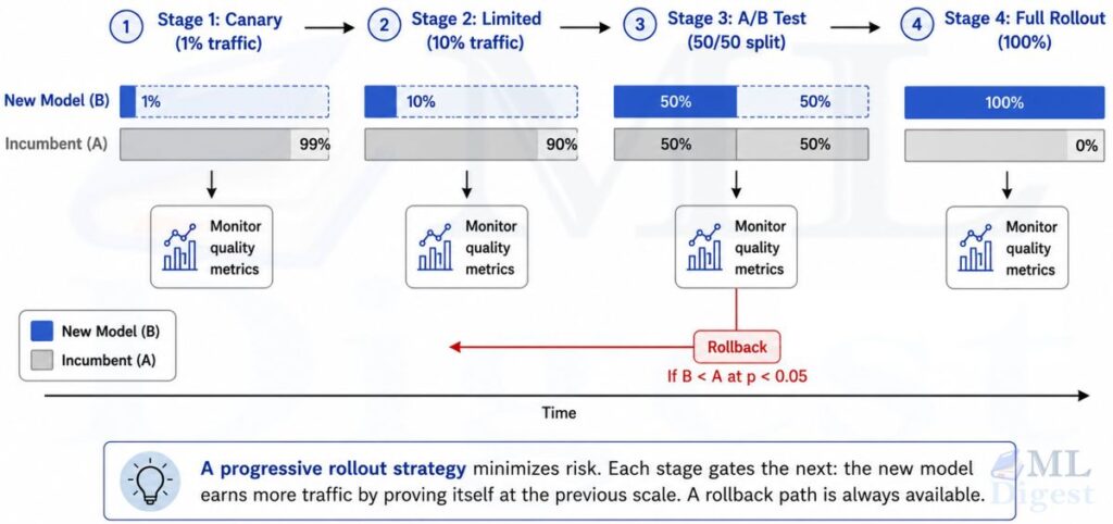
The traffic-splitting logic at the heart of an A/B router is simple but has one important requirement: each user must always be sent to the same model variant throughout the experiment, otherwise the same person might see two different model personalities in one session, corrupting the quality signal. The standard solution is to hash the user ID together with an experiment identifier and use the resulting number to make a deterministic assignment. A user whose hash falls below a threshold goes to variant B; everyone else goes to variant A. The threshold is set to match your desired traffic split — 50% for a balanced A/B test, lower for a cautious canary. Every routed request is logged with its variant label so that quality scores can later be grouped and compared. Once enough requests have accumulated for the difference to be statistically significant, you either promote variant B to 100% of traffic or roll it back entirely.
The minimum viable safe-deployment checklist for any model update:
- Tag the new artifact with a version string and store its eval scores.
- Deploy to 1-5% canary traffic. Monitor for 24-48 hours.
- If canary metrics are healthy, ramp to 50% for an A/B test until statistical significance is reached.
- If A/B results favor the new version, complete the rollout. If not, drain traffic to the incumbent.
- Keep the previous version’s artifacts and infrastructure live for at least one rollback window (typically 72 hours) after full rollout.
5. Putting It All Together: A Decision Framework
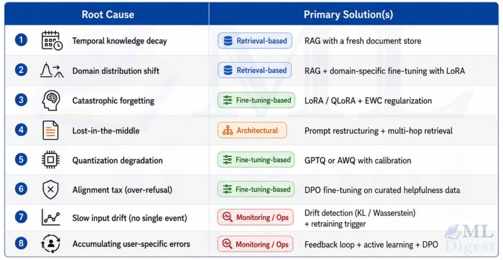
The diagram below maps each failure mode to the recommended solution. In practice, multiple failure modes can co-occur, and the solutions are composable.
Here is a condensed decision tree for the engineer facing an underperforming model:
%%{init: {'theme': 'base', 'themeVariables': {
    'fontSize': '28px',
    'fontFamily': 'Arial',
    'primaryTextColor': '#000000'
}}}%%

flowchart TD
    START([LLM outputs have degraded]) --> Q1{Recent facts or<br>new domain knowledge?}
    Q1 -->|YES| A1[Deploy RAG.<br>Update your document store regularly.]
    Q1 -->|NO| Q2{Appeared after<br>a fine-tuning run?}
    Q2 -->|YES| A2[Switch to LoRA.<br>Add EWC if forgetting persists.]
    Q2 -->|NO| Q3{Appeared after model<br>compression or quantization?}
    Q3 -->|YES| A3[Re-quantize using GPTQ or AWQ<br>with a proper calibration set.]
    Q3 -->|NO| Q4{Worse on long-document<br>or multi-document tasks?}
    Q4 -->|YES| A4[Restructure prompts: key info first/last.<br>Consider multi-hop retrieval.]
    Q4 -->|NO| Q5{Alignment fine-tuning<br>preceded the degradation?}
    Q5 -->|YES| A5[Audit refusal patterns.<br>Fine-tune on helpfulness data with DPO.]
    Q5 -->|NO| Q6{Gradual with no<br>single triggering event?}
    Q6 -->|YES| A6[Run KL / Wasserstein drift detection.<br>If drift confirmed → trigger incremental retraining.]
    Q6 -->|NO| Q7{Users repeatedly correcting<br>or reformulating responses?}
    Q7 -->|YES| A7[Build a feedback loop.<br>Use active learning + DPO fine-tune.]
    Q7 -->|NO| A8[Audit your deployment pipeline.<br>Roll back to last known-good version.]
Summary
LLM performance degradation is not a single bug but a family of problems, each with a distinct root cause and a targeted solution. The key takeaways are:
- Temporal knowledge decay is ubiquitous and best addressed by RAG: keep the model’s weights frozen and let a retrieval system supply fresh facts.
- Catastrophic forgetting is the hidden cost of fine-tuning. Parameter-efficient methods like LoRA minimize this by changing only a tiny fraction of weights.
- Quantization trades accuracy for efficiency. Calibrated methods like GPTQ and AWQ recover most of that lost accuracy with only minutes of extra work.
- Long-context degradation is a real architectural limitation. Restructure your prompts and consider multi-hop retrieval before assuming the model is broken.
- Slow drift is the silent killer. Track KL divergence or Wasserstein distance on rolling windows of input embeddings to catch it before it becomes user-visible.
- Feedback loops and active learning turn deployment into a continuous improvement cycle. Prioritize the most uncertain examples for labeling and use preference data to run DPO fine-tunes.
- Safe deployment (versioning, canary rollouts, A/B testing) gives you the ability to catch regressions before they affect all users and roll back instantly when they do.
- Monitoring is what separates teams that catch degradation early from those who learn about it from angry users. A 1% sampling pipeline with an LLM-as-judge is the minimum viable safeguard.

Silpa brings 5 years of experience in working on diverse ML projects, specializing in designing end-to-end ML systems tailored for real-time applications. Her background in statistics (Bachelor of Technology) provides a strong foundation for her work in the field. Silpa is also the driving force behind the development of the content you find on this site.

Happy is a seasoned ML professional with over 15 years of experience. His expertise spans various domains, including Computer Vision, Natural Language Processing (NLP), and Time Series analysis. He holds a PhD in Machine Learning from IIT Kharagpur and has furthered his research with postdoctoral experience at INRIA-Sophia Antipolis, France. Happy has a proven track record of delivering impactful ML solutions to clients. Check more about him here: https://sites.google.com/site/slhappyin/
Subscribe to our newsletter!