Consider a spam filter trained in 2010. By 2020, users receive far more promotional newsletters than before. The types of emails changed, but what counts as spam stayed the same. That is data drift. Meanwhile, scammers have learned to mimic legitimate writing, so emails that look friendly are now malicious. The same kind of email now deserves a different label. That is concept drift.
People often treat these two problems as interchangeable, but operationally they are different failure modes. Data drift asks whether the incoming data no longer looks like the data used to build the model. Concept drift asks whether the relationship between the inputs and the target has changed. One can happen without the other, and the right response depends on which one you are facing.
In practice, this distinction matters because not every drift alert means your model is wrong, and not every model failure is visible from feature histograms alone. In this article, I will build the intuition first, then formalize the math, show how to detect each type of drift, and finish with a runnable Python example.
1. Why the distinction matters
1.1 Same alert category, different operational meaning
Suppose you are monitoring a fraud model, such as one in a real-time fraud detection system.
- If transaction amounts, merchant categories, or geographic patterns shift, you may have data drift.
- If fraudsters start mimicking legitimate customer behavior more effectively, you may have concept drift.
The first case says, “the world looks different.” The second case says, “the world behaves differently.”
Those are not the same engineering problem:
- Data drift can be harmless if the model still generalizes well.
- Concept drift is dangerous because the learned decision rule itself becomes stale.
- A model can fail badly under concept drift even when simple feature-level drift checks remain quiet.
1.2 Why teams confuse them
Most production ML systems only see features immediately. Labels often arrive hours, days, or weeks later. That means data drift is easier to detect than concept drift. Teams end up using feature drift as a proxy for model health because it is available, not because it is sufficient. That delay problem is also one reason point-in-time correctness matters so much in monitoring and evaluation pipelines.
This is one of the most common monitoring mistakes I see in practice. A dashboard full of shifted feature distributions can create panic even when the model remains accurate. At the same time, a perfectly calm feature dashboard can hide a collapsing predictor when the target mechanism changes.
1.3 A compact comparison
| Data drift | Concept drift | |
|---|---|---|
| What changed? | Input distribution $P_t(X)$ | Target relationship $P_t(Y \mid X)$ |
| Detectable without labels? | Often yes | Usually no |
| Typical symptom | Shifted features, changed missingness, range violations, or embedding spread | Worsening accuracy, AUC, calibration, or residual behavior |
| Common response | Pipeline checks, reference-window updates, recalibration, or selective retraining | Fresh labeled data, retraining, revised feature representation, or policy update |
2. The formal definitions
2.1 Start from the data-generating process
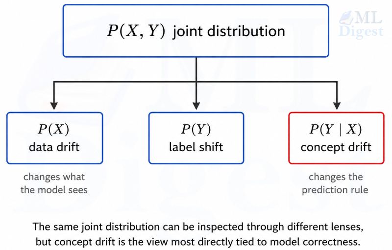
Let $X$ denote the input features and $Y$ the target. At time $t$, the world defines a joint distribution:
$$
P_t(X, Y)
$$
If your training data came from a reference period $r$, then your model was effectively built under $P_r(X, Y)$. Drift means that the production-time distribution is no longer the same, i.e., $P_t(X, Y) \neq P_r(X, Y)$.
The important point is that the joint distribution can change in multiple ways.
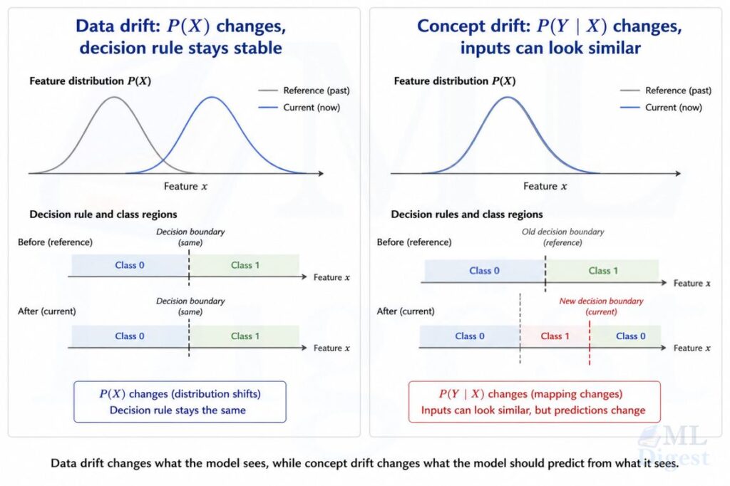
2.2 Data drift
Data drift usually means the marginal distribution of features changes:
$$
P_t(X) \neq P_r(X)
$$
In production discussions, this is often called covariate drift. The stricter textbook term covariate shift usually refers to the narrower case where $P_t(X)$ changes while the conditional target rule stays fixed, i.e., $P_t(Y \mid X) = P_r(Y \mid X)$.
Examples:
- A recommender system suddenly receives many more mobile users than desktop users.
- A medical model receives data from a new hospital with different scanners and slightly different measurement ranges.
2.3 Concept drift
Concept drift means the conditional relationship between inputs and target changes:
$$
P_t(Y \mid X) \neq P_r(Y \mid X)
$$
This is the more serious failure mode for predictive performance because it changes what the correct prediction should be for the same type of input.
Examples:
- A spam filter sees the same vocabulary, but the words associated with spam change.
- A credit-risk model faces new lending behavior after a policy change.
- A predictive maintenance model sees the same sensors, but a newly installed part changes what vibration patterns indicate failure.
2.4 Related shifts that often appear nearby
You will also encounter:
- Label shift (or class-prior shift): $P_t(Y) \neq P_r(Y)$. This is especially impactful in systems already managing class imbalance, where a rare class can vanish from short monitoring windows entirely.
These categories can overlap. In the classical label-shift setup, $P_t(X \mid Y)$ stays roughly fixed while class prevalences change. In production, real systems often exhibit more than one form of change at once.
2.5 Why the boundary between them gets blurry
By Bayes’ rule,
$$
P_t(Y \mid X) = \frac{P_t(X \mid Y) P_t(Y)}{P_t(X)}
$$
This identity explains why people blur the categories. A shift in one part of the distribution can propagate to another view of the same problem. But operationally, the monitoring question is still useful:
- Are the inputs changing?
- Is the prediction rule changing?
That framing helps decide what to measure and what action to take.
3. Intuition through examples
3.1 Data drift without concept drift
Imagine a classifier that predicts whether an ecommerce order will be returned. During training, most orders come from domestic shipping zones. Later, the company expands internationally, and package weights, shipping times, and duties change their distributions. If the basic return logic still holds, then the model may still perform well after recalibration or mild retraining.
The world looks different, but the rule has not fundamentally changed.
3.2 Concept drift without obvious data drift
Now imagine the same return model during a policy change. The company introduces free returns for premium customers. The feature distribution may look almost unchanged, but the same customer profile now leads to a different probability of return.
That is concept drift. Histograms might not save you here.
3.3 Both can happen together
This is the most realistic case. In fraud detection, new transaction patterns may appear at the same time that adversaries discover new attack strategies. Your features drift, and the target relationship drifts with them.
When both happen, it is easy to overreact to the visible part, namely the feature shift, and miss the deeper issue, namely that yesterday’s decision surface no longer reflects today’s environment.
3.4 Concept drift in wealth classification
A model trained in 1900 to classify wealth from annual income might have labeled \$5,000 per year as “wealthy.” Reuse that threshold today and the mapping from income to the label “wealthy” is badly outdated because inflation and living standards have changed. The feature value has not changed, but the label it should produce for that same numeric income can flip. That is $P_t(Y \mid X)$ shifting due to a changing economic context, not merely a change in the people being observed.
Notice that a feature-drift monitor would not save you in the frozen-input thought experiment. If you replayed the same 1900 income values, the feature distribution would look stable and a pure input-drift alarm could stay quiet, even though the old decision rule would now be systematically misaligned with the intended label. Only labeled performance monitoring, policy review, or refreshed supervision would reveal that problem.
In the realistic scenario, income values collected today are also distributed completely differently from 1900 data — the mean has shifted by roughly two orders of magnitude and the variance has expanded enormously. So both drift types compound: $P_t(X)$ changed and $P_t(Y \mid X)$ changed. Any domain where the underlying scale of measurement shifts over time is likely to exhibit this combination.

4. How to detect data drift
4.1 Start with simple distribution checks
For tabular features, the first line of defense is often univariate monitoring:
- mean, median, and standard deviation shifts
- missing-value rate changes
- category frequency changes
- range violations and schema mismatches
These checks catch many real deployment issues because a surprising amount of “drift” is actually caused by upstream data bugs, unit changes, broken joins, or default values leaking into production.
4.2 Statistical distance measures
For numeric features, common drift measures include the Kolmogorov-Smirnov test, Kullback-Leibler divergence, and Jensen-Shannon divergence. In business monitoring, teams also use Population Stability Index (PSI).
One common PSI form is:
$$
\mathrm{PSI} = \sum_{i=1}^{B} (q_i – p_i) \ln\left(\frac{q_i}{p_i}\right)
$$
where $p_i$ is the reference fraction in bin $i$ and $q_i$ is the current fraction.
PSI is easy to compute and easy to explain, but it depends on your binning strategy. It is best treated as a monitoring heuristic, not as a universal law.
For continuous distributions, a more information-theoretic measure is Jensen-Shannon divergence:
$$
\mathrm{JS}(P, Q) = \frac{1}{2} \mathrm{KL}(P \parallel M) + \frac{1}{2} \mathrm{KL}(Q \parallel M), \quad M = \frac{1}{2}(P + Q)
$$
It is symmetric and often easier to work with than plain KL divergence.
4.3 Multivariate and representation-based checks
Univariate tests can miss joint changes. If each feature moves a little, but the feature combination changes substantially, separate histograms may look fine while the geometry of the data cloud has shifted.
That is why mature monitoring systems also use:
- embedding-distance monitoring
- multivariate two-sample tests
- slice-based checks by country, device, cohort, or product line
- joint monitoring of input feature distributions and model output score distributions
For streaming settings, tools like River support online monitoring and adaptive estimators. For batch production systems, open-source libraries such as Evidently AI and NannyML provide pre-built monitors for feature drift, data quality, and, in some setups, performance estimation without immediate access to fresh labels. If you also need a broader framing for unusual or out-of-distribution inputs, the related anomaly detection overview is a useful companion.
5. How to detect concept drift
5.1 Performance monitoring is the core signal
Concept drift is fundamentally about prediction quality under a changing world. So the most direct signal is performance over time, using the same kinds of metrics discussed in evaluation metrics in machine learning:
- rolling accuracy, precision, recall, F1, or AUC for classification
- rolling MAE, RMSE, or MAPE for regression
- calibration drift, especially for risk scores and probabilities; if that is a new topic, see model calibration
- residual drift for time series forecasting and regression
If labels arrive with delay, maintain time-indexed evaluation windows and monitor the freshest labeled slice you can obtain.
A simple rolling loss statistic is:
$$
L_t = \frac{1}{w} \sum_{i=t-w+1}^{t} \ell(\hat{y}_i, y_i)
$$
where $w$ is the window size and $\ell$ is the task-specific loss.
If $L_t$ rises persistently beyond normal variation, you have evidence that the model’s mapping is becoming stale.
5.2 Change detectors for streams
In online learning and stream mining, change detectors such as DDM, ADWIN, and Page-Hinkley are commonly used.
The intuition is simple:
- track a statistic such as error rate or mean loss
- compare recent behavior against earlier behavior
- trigger a warning or change signal when the difference is too large to be explained by routine noise
These detectors are useful, but they are not magic. They work on observable sequences, usually errors or loss, which means they are only as good as the signals you feed them.
5.3 Why labels are the bottleneck
Data drift can often be monitored immediately. Concept drift often cannot. If your labels arrive after a customer churn cycle, a clinical review, or a manual fraud investigation, then concept drift may be discovered late.
That is why strong production systems combine:
- fast unlabeled monitoring for input changes
- delayed labeled monitoring for actual model quality
- champion-challenger models
- periodic relabeling, active sampling, or synthetic data generation for fresh ground truth
In mature teams, these loops are usually embedded in a wider MLOps process rather than handled as one-off dashboard checks.
6. A practical Python example
6.1 What we will simulate
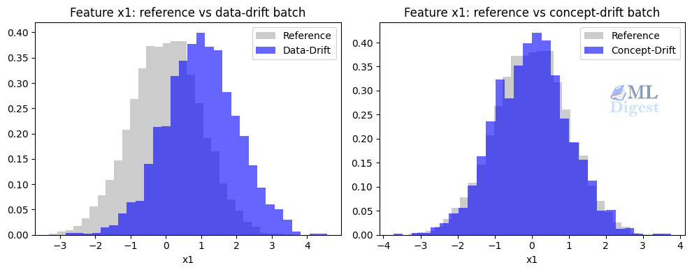
We will create three batches:
- A reference batch used to train a logistic regression classifier.
- A current batch with data drift only, where a feature distribution shifts but the label rule stays the same.
- A current batch with concept drift only, where the label rule changes but the feature distribution stays roughly the same.
This setup is intentionally simple because the goal is not to build a perfect detector. The goal is to make the distinction visible in code.
6.2 Runnable example
import numpy as np
import pandas as pd
from scipy.special import expit
from scipy.stats import ks_2samp
from sklearn.linear_model import LogisticRegression
from sklearn.metrics import accuracy_score, roc_auc_score
rng = np.random.default_rng(42)
def make_batch(n, x1_mean=0.0, beta=(2.0, -1.0), intercept=0.0):
x1 = rng.normal(loc=x1_mean, scale=1.0, size=n)
x2 = rng.normal(loc=0.0, scale=1.0, size=n)
logits = intercept + beta[0] * x1 + beta[1] * x2
probs = expit(logits)
y = rng.binomial(1, probs, size=n)
return pd.DataFrame({"x1": x1, "x2": x2, "y": y})
def psi(reference, current, bins=10, eps=1e-6):
edges = np.quantile(reference, np.linspace(0, 1, bins + 1))
edges[0] = -np.inf
edges[-1] = np.inf
ref_hist, _ = np.histogram(reference, bins=edges)
cur_hist, _ = np.histogram(current, bins=edges)
ref_frac = np.clip(ref_hist / ref_hist.sum(), eps, None)
cur_frac = np.clip(cur_hist / cur_hist.sum(), eps, None)
return np.sum((cur_frac - ref_frac) * np.log(cur_frac / ref_frac))
def evaluate(model, batch, name):
X = batch[["x1", "x2"]]
y = batch["y"]
prob = model.predict_proba(X)[:, 1]
pred = (prob >= 0.5).astype(int)
print(f"{name}")
print(f" accuracy: {accuracy_score(y, pred):.3f}")
print(f" roc_auc : {roc_auc_score(y, prob):.3f}")
# 1) Reference data and model training
reference = make_batch(n=5000, x1_mean=0.0, beta=(2.0, -1.0))
model = LogisticRegression(max_iter=1000)
model.fit(reference[["x1", "x2"]], reference["y"])
# 2) Data drift only: input distribution changes, target rule stays the same
data_drift_batch = make_batch(n=2000, x1_mean=1.0, beta=(2.0, -1.0))
# 3) Concept drift only: input distribution stays similar, target rule changes
concept_drift_batch = make_batch(n=2000, x1_mean=0.0, beta=(-2.0, -1.0))
# Drift checks on x1
psi_data = psi(reference["x1"].to_numpy(), data_drift_batch["x1"].to_numpy())
psi_concept = psi(reference["x1"].to_numpy(), concept_drift_batch["x1"].to_numpy())
ks_data = ks_2samp(reference["x1"], data_drift_batch["x1"])
ks_concept = ks_2samp(reference["x1"], concept_drift_batch["x1"])
print("Feature drift on x1")
print(f" PSI(reference, data_drift_batch) = {psi_data:.3f}")
print(f" PSI(reference, concept_drift_batch) = {psi_concept:.3f}")
print(f" KS p-value (data drift batch) = {ks_data.pvalue:.6f}")
print(f" KS p-value (concept drift batch) = {ks_concept.pvalue:.6f}")
print()
# Performance checks
evaluate(model, reference, "Reference batch")
evaluate(model, data_drift_batch, "Data-drift-only batch")
evaluate(model, concept_drift_batch, "Concept-drift-only batch")
# Expected output:
# Feature drift on x1
# PSI(reference, data_drift_batch) = 0.975
# PSI(reference, concept_drift_batch) = 0.005
# KS p-value (data drift batch) = 0.000000
# KS p-value (concept drift batch) = 0.687661
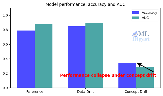
# Reference batch
# accuracy: 0.796
# roc_auc : 0.881
# Data-drift-only batch
# accuracy: 0.844
# roc_auc : 0.885
# Concept-drift-only batch
# accuracy: 0.353
# roc_auc : 0.2896.3 How to read the result
You should typically observe the following pattern:
- The data-drift batch shows a stronger PSI and a smaller KS p-value for
x1. - The concept-drift batch shows much weaker feature drift on
x1. - The model performance stays relatively stable on the data-drift-only batch.
- The model performance degrades sharply on the concept-drift-only batch.
That is the lesson in one screenful of code: feature drift metrics and model performance metrics answer different questions.
6.4 What this example leaves out
Real systems are more complicated.
- Drift can occur in multiple features at once.
- Labels can be delayed and noisy.
- Retraining can change the feature distribution seen by downstream models.
- Feedback loops can make drift partly self-inflicted.
Still, the example is useful because it demonstrates the most important operational truth: concept drift is about a changing predictive relationship, not merely a changing input histogram.
7. What to do when drift is detected
7.1 If you detect data drift
Do not jump straight to retraining. First check whether the shift reflects:
- a broken upstream pipeline
- a benign seasonal change
- a known business event such as a launch or promotion
- a shift concentrated in one slice rather than the full population
Then answer the practical question: did model quality actually move?
If performance is stable, the right response may be to update monitoring thresholds, refresh your reference window, recalibrate probabilities, or collect more recent training data for a later refresh.
7.2 If you detect concept drift
Treat it as a model-validity issue.
- Inspect the freshest labeled errors; SHAP values can surface which features are most responsible for unexpected predictions and help confirm whether the learned associations have shifted.
- Check whether the label definition or business policy changed.
- Retrain on newer labeled data if the target rule truly moved.
- Revisit features if the old representation no longer captures the new mechanism.
- Consider adaptive or online-learning strategies if the environment changes continuously, especially if you expect repeated refresh cycles similar to continuous learning.
For some systems, threshold tuning alone is not enough. If the mapping from features to label has changed materially, you need new supervision, not just new calibration.
7.3 Best practices that save time
- Monitor both unlabeled feature drift and labeled performance drift.
- Keep reference windows explicit, versioned, and time-bounded.
- Track drift by slice, not just globally.
- Pair drift alerts with business-context annotations.
- Separate data-quality failures from real population shifts.
- Log prediction scores, features, model version, and eventual labels so postmortems are possible.
Summary
Data drift means the input distribution changes. Concept drift means the predictive relationship changes. The first tells you that the model is seeing a different world. The second tells you that the model may have learned the wrong rule for the current world.
If you remember one practical rule, make it this: monitor feature shift to know when the environment is moving, and monitor labeled performance to know when the model is no longer correct. Those two signals complement each other, and neither one is enough by itself.

Silpa brings 5 years of experience in working on diverse ML projects, specializing in designing end-to-end ML systems tailored for real-time applications. Her background in statistics (Bachelor of Technology) provides a strong foundation for her work in the field. Silpa is also the driving force behind the development of the content you find on this site.

Happy is a seasoned ML professional with over 15 years of experience. His expertise spans various domains, including Computer Vision, Natural Language Processing (NLP), and Time Series analysis. He holds a PhD in Machine Learning from IIT Kharagpur and has furthered his research with postdoctoral experience at INRIA-Sophia Antipolis, France. Happy has a proven track record of delivering impactful ML solutions to clients.
Subscribe to our newsletter!