Imagine asking a librarian for one page that proves a claim. The librarian first runs through the whole building and places 100 possibly useful books on a cart. That first pass must be fast, so a few books are merely about the right topic. A careful second pass opens the most promising books, reads the relevant passages alongside your question, and moves the best evidence to the top. In retrieval-augmented generation (RAG), reranking is that careful second pass.
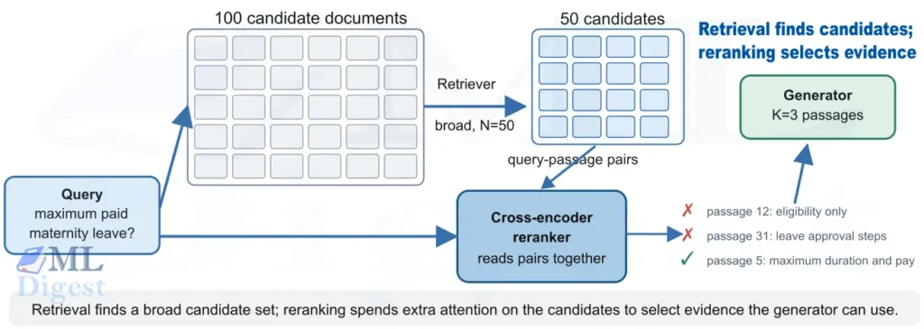
A retriever is optimized to find a broad candidate set cheaply. A reranker spends more computation comparing the query with each candidate and can improve their order.
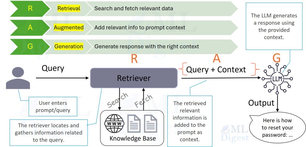
When the candidate set contains the needed evidence, this architectural addition can improve answer grounding without simply increasing the generator’s context window. For a broader introduction to the full pipeline, see Retrieval-Augmented Generation. For guidance on deciding whether retrieval is the right tool at all, see When to Use RAG.
1. Why top-$k$ retrieval is not enough
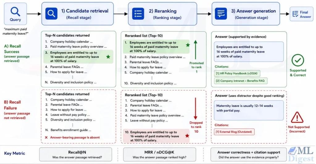
Retrieval is a recall problem before it is a ranking problem. Its first objective is to place at least one passage containing the needed evidence somewhere in the candidate list. Its second objective, putting that passage first, is much harder.
Consider the query: “What is the maximum maternity leave paid by the policy?” A vector retriever may return passages about parental benefits, leave approval, sick leave, and a policy revision. All are semantically related. Only one passage states the maximum duration and payment condition. If that passage is ranked tenth, a generator given the first five chunks may confidently answer from weaker evidence.
This failure is common because dense retrieval normally scores two texts independently. It produces a query vector $q$ and a vector $v_i$ for each document $d_i$, then uses a similarity function such as cosine similarity:
$$
s_{bi}(q, d_i) = \frac{q \cdot v_i}{\lVert q \rVert_2 \lVert v_i \rVert_2}
$$
That single similarity value has to represent every useful relation between a query and a passage. It can recognize that “maternity leave” and “parental benefits” belong together, but it may not reliably distinguish “maximum paid duration” from a passage that only describes eligibility. Keyword retrieval such as BM25 has the complementary weakness: it handles exact terms well but can miss synonyms, paraphrases, and other cases with little lexical overlap.
Top-$k$ makes the trade-off visible:
- A small $k$ keeps latency and prompt cost low, but can exclude the answer-bearing passage.
- A large $k$ increases recall, but supplies the generator with redundant, contradictory, or tangential context.
- More context is not automatically better context. Distractor passages can cause the model to cite the wrong fact, combine incompatible conditions, or ignore the evidence altogether.
Reranking lets the system retrieve generously, then select sparingly. A typical configuration retrieves $N=50$ to $200$ candidates, reranks those candidates, and supplies only $K=3$ to $10$ well-chosen passages to the generator.
2. The reranking objective
Let $C_N(q)$ be the $N$ candidates returned by the first-stage retriever for query $q$. A reranker assigns each candidate $d_i$ a relevance score:
$$
s(q, d_i) = f_\theta(q, d_i), \qquad d_i \in C_N(q)
$$
The system sorts by $s$ and returns the first $K$ passages:
$$
R_K(q) = \operatorname{TopK}_{d_i \in C_N(q)} s(q, d_i)
$$
Unlike the bi-encoder score, $f_\theta$ may inspect individual query tokens and passage tokens together. It can reward a passage for containing the answer to the specific relation being asked, not just for sharing a topic.
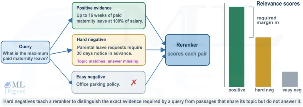
Labeled triples $(q, d_i^+, d_j^-)$ are commonly used during training of this model, where $d_i^+$ is relevant and $d_j^-$ is not. A pairwise margin loss expresses the desired ordering:
$$
\mathcal{L}_{pair} = \max\left(0, m – s(q,d_i^+) + s(q,d_j^-)\right)
$$
Here $m$ is a margin. The loss is zero only when the positive passage scores at least $m$ above the negative one. In practice, hard negatives matter greatly: a passage that looks relevant but fails one required constraint teaches more than an obviously unrelated paragraph. For a broader introduction to training objectives, see Neural Network Loss Functions. The MS MARCO passage-ranking dataset is a widely used source of query-passage supervision and benchmark evaluation.
The score itself is usually meaningful only for ordering candidates for the same query. A score of 3.2 for one query is not necessarily more trustworthy than 1.7 for another. Do not treat raw reranker scores as calibrated probabilities unless you explicitly calibrate them. See Model Calibration for the distinction between ranking confidence and probability estimates.
3. Bi-encoders and cross-encoders
3.1 Bi-encoders: fast independent representations
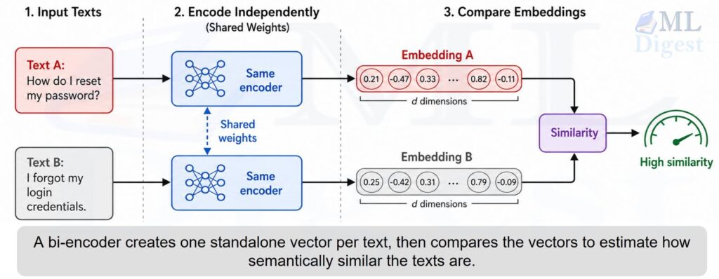
A bi-encoder encodes queries and documents separately:
$$
q = E_q(\text{query}), \qquad v_i = E_d(d_i)
$$
The document vectors $v_i$ can be computed once and stored in an approximate-nearest-neighbor index. At query time, the system computes one query vector and finds nearby document vectors. This lookup is conceptually a nearest-neighbor search; K-Nearest Neighbors (KNN) explains the underlying neighborhood idea, while approximate indexes make the lookup practical at large scale. This is why bi-encoders scale to millions or billions of passages.
Their limitation is deliberate: while generating $v_i$ for document $d_i$, the document encoder cannot see the user’s query. As a result, the query and passage interact only when their final vectors are compared.
3.2 Cross-encoders: detailed pairwise judgment
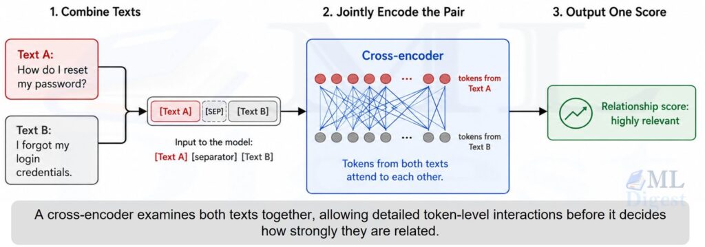
A cross-encoder concatenates the query and passage into one transformer input:
$$
x_i = [\mathrm{CLS}]\ q\ [\mathrm{SEP}]\ d_i\ [\mathrm{SEP}]
$$
Self-attention allows every query token to attend to every passage token. A scoring/classification head converts the final representation into a relevance score, often a logit. This approach was popularized for passage reranking by Nogueira and Cho, whose BERT reranker showed that transformer interaction can substantially improve ranking quality.
For the leave-policy question, the token “maximum” can attend directly to “up to 16 weeks” and “paid” can attend directly to “at 100% of salary.” A passage that says “employees may request leave” shares topical words but lacks the needed relationship, so it receives a lower score.
The cost is that every pair must be processed at query time. If $L_q$ and $L_{d_i}$ are query and document lengths, full self-attention is roughly quadratic in the combined length, $O((L_q + L_{d_i})^2)$, per candidate. Cross-encoders are therefore commonly used as rerankers, but are typically unsuitable as first-stage retrievers over a large corpus.
3.3 Choosing between them
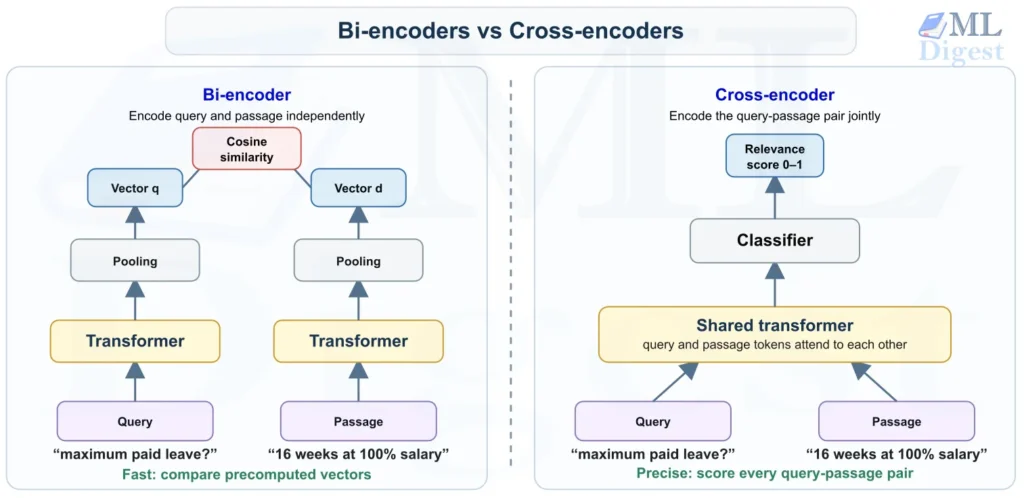
| Property | Bi-encoder | Cross-encoder |
|---|---|---|
| Encodes query and passage | Separately | Together |
| Corpus indexing | Precompute passage vectors | Cannot precompute pair representations |
| Query-time work | One query embedding plus vector search | One forward pass per candidate pair |
| Best role | First-stage retrieval | Second-stage reranking |
| Interaction quality | Compressed into embedding similarity | Token-level query-passage attention |
| Typical scale | Whole corpus | Top tens or hundreds of candidates |
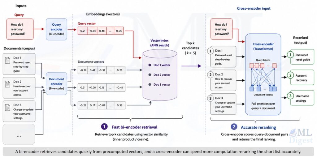
The practical answer is usually not “bi-encoder or cross-encoder.” It is bi-encoder then cross-encoder. A lexical retriever can also join the first stage, producing a hybrid candidate set. This protects against both semantic misses and exact-term misses.
4. Late interaction: a middle ground
Late-interaction models preserve more information than a single-vector bi-encoder without paying the full cost of a cross-encoder. ColBERT, short for Contextualized Late Interaction over BERT, is the classic example.
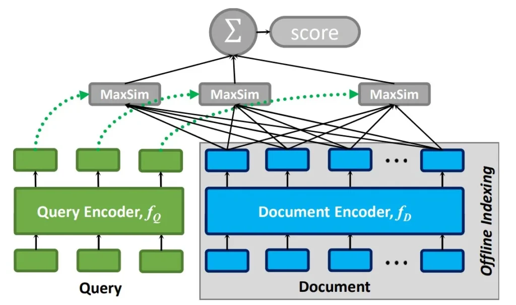
Instead of one vector, ColBERT produces a vector for every query token and every token in a document. It encodes queries and documents independently, so document token embeddings can be indexed ahead of time.
Let $d_x$ be the $x$-th document, let $q^i$ be the $i$-th query token, and let $d_x^j$ be the $j$-th token in $d_x$. For each query token $q^i$, MaxSim keeps only its strongest match among the tokens in $d_x$:
$$
\operatorname{MaxSim}(q^i, d_x) = \max_{j=1}^{|d_x|} E_q(q^i) \cdot E_d(d_x^j)
$$
The final score adds those best matches across the whole query:
$$
s_{late}(q,d_x) = \sum_{i=1}^{|q|} \operatorname{MaxSim}(q^i, d_x)
$$
In simpler terms, take one query token at a time. Tokens can be whole words or subword pieces; BERT-family encoders commonly use WordPiece tokenization. Compare it with every document token, keep the highest similarity, and ignore the weaker matches for that query token. Repeat for every query token, then add the kept scores.
For example, a token representing “maximum” may find its best match among the tokens around “up to 16 weeks,” while “paid” may match tokens around “100% of salary.” Each token contributes its own best evidence. For a multi-term query, a document will typically score well when it contains strong matches for several important query tokens, rather than only one related word.
Here, $E_q(q^i)$ is the vector for query token $q^i$, $E_d(d_x^j)$ is the vector for token $d_x^j$ in document $d_x$, and their dot product measures similarity. The model can therefore preserve evidence for several distinct query terms, such as an entity, a time constraint, and a requested property.
Late interaction creates a useful middle point:
- It has richer token-level matching than a one-vector bi-encoder.
- It can precompute document-side representations, unlike a cross-encoder.
- It uses more storage and more query-time computation than a standard dense retriever.
- It still lacks the full joint attention of a cross-encoder, so subtle reasoning across the entire pair can remain difficult.
Use it when a plain embedding retriever loses too much fine-grained signal and cross-encoding every candidate violates the latency budget. The ColBERT documentation provides an implementation-oriented starting point.
5. A production retrieval and reranking pipeline
A robust pipeline separates candidate generation, precision ranking, and evidence packaging.
5.1 Retrieve broadly and diversify
First, retrieve candidates from one or more indexes. A hybrid setup can union dense and BM25 results, then remove duplicate chunk IDs. If the corpus contains near-duplicate chunks from a long document, consider diversity methods such as maximal marginal relevance (MMR) before or after reranking.
Do not let candidate generation become too narrow. A reranker cannot rescue an answer passage that it never sees. Diagnose retrieval recall separately from reranking quality.
5.2 Rerank with the original user question
Pass the original question, not only a compressed keyword query, to the reranker. The entire wording often carries the constraint that distinguishes the correct passage. If query rewriting is used, retain the original query and test both formulations.
For long documents, rerank chunks rather than whole documents, but preserve metadata linking each chunk to its source. A reranker’s maximum input length applies to the combined query, passage, and special tokens; it is often 512 subword tokens for BERT-derived models, but model limits differ. Careless chunk construction can therefore truncate the decisive sentence. Chunk at coherent boundaries, include a small overlap when necessary, and place a useful title or section heading with each chunk. These document-ingestion choices set the upper bound on evidence that any retriever or reranker can recover.
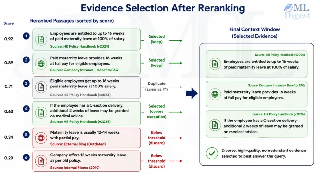
5.3 Select the final evidence set
After ranking, selection is more than taking the first $K$ rows:
- Start with $K=3$ to $5$. This is a sensible baseline for concise question answering.
- Remove duplicates. Several overlapping chunks that state the same fact waste context capacity.
- Enforce diversity when needed. For multi-part questions, select passages that cover different subquestions or sources.
- Apply a confidence policy. If the top score is below a query-specific or calibrated threshold, ask for clarification, broaden retrieval, or answer that the evidence is insufficient.
- Keep provenance. Send source IDs, titles, and offsets alongside text so the generator can cite evidence and a user can inspect it.
For open-ended synthesis, a larger $K$ may help, but use a token budget rather than a fixed document count. Allocate space to the highest-quality nonredundant passages. Reranking is a ranking method, not a guarantee that every retained passage is factually correct or current.
6. A runnable Python implementation
The Sentence Transformers library provides a simple interface for both embedding models and cross-encoder rerankers. The example below uses a bi-encoder for first-stage candidate generation and cross-encoder/ms-marco-MiniLM-L-6-v2 for the second stage. It is suitable for a small in-memory demonstration. In production, replace the NumPy search with a persistent vector database or ANN index.
# pip install sentence-transformers numpy

from sentence_transformers import CrossEncoder, SentenceTransformer
import numpy as np

documents = [
    {
        "id": "policy-1",
        "text": "Eligible birth parents receive up to 16 weeks of paid maternity leave at 100% of base salary.",
    },
    {
        "id": "policy-2",
        "text": "Employees must submit parental leave requests at least 30 days before the planned start date.",
    },
    {
        "id": "policy-3",
        "text": "Adoptive parents may receive up to 12 weeks of paid parental leave after placement.",
    },
    {
        "id": "policy-4",
        "text": "Sick leave is available for qualifying medical conditions and is separate from parental leave.",
    },
    {
        "id": "policy-5",
        "text": "Employees on maternity leave continue to receive health insurance under the usual contribution rules.",
    },
]

query = "What is the maximum paid maternity leave?"

# First stage: encode documents once. normalize_embeddings=True makes a dot
# product equivalent to cosine similarity for these unit-length vectors.
embedder = SentenceTransformer("all-MiniLM-L6-v2")
document_texts = [document["text"] for document in documents]
document_vectors = embedder.encode(document_texts, normalize_embeddings=True)
query_vector = embedder.encode(query, normalize_embeddings=True)

# Retrieve more than the generator will see. For a real corpus, use ANN search.
retrieve_top_n = 4
retrieval_scores = document_vectors @ query_vector
candidate_indices = np.argsort(retrieval_scores)[::-1][:retrieve_top_n]
candidates = [documents[index] for index in candidate_indices]

# Second stage: jointly score every (query, candidate) pair.
reranker = CrossEncoder("cross-encoder/ms-marco-MiniLM-L-6-v2")
pairs = [(query, candidate["text"]) for candidate in candidates]
rerank_scores = reranker.predict(pairs)

# Keep original metadata and sort by the more precise reranker score.
ranked = sorted(
    zip(candidates, rerank_scores), key=lambda item: item[1], reverse=True
)

final_top_k = 3
for rank, (document, score) in enumerate(ranked[:final_top_k], start=1):
    print(f"{rank}. score={score:.3f} source={document['id']}")
    print(f"   {document['text']}")
# Expected output:
#     1. score=4.322 source=policy-1
#     Eligible birth parents receive up to 16 weeks of paid maternity leave at 100% of base salary.
#     2. score=-2.425 source=policy-3
#     Adoptive parents may receive up to 12 weeks of paid parental leave after placement.
#     3. score=-4.079 source=policy-5
# Employees on maternity leave continue to receive health insurance under the usual contribution rules.The cross-encoder output is a ranking score, not an answer. The code intentionally exposes both stages so that they can be evaluated independently. Log the candidate IDs before and after reranking. When an answer is wrong, this log answers a crucial debugging question: did retrieval miss the evidence, or did reranking demote it? For a broader operational workflow, see Debugging a RAG Workflow.
Batched inference for real traffic
The code above scores one query. For a service, batch candidate pairs across requests where latency permits, use GPU inference, and cap maximum sequence length deliberately. A simple request shape is:
retrieve N candidates -> deduplicate -> rerank in batches -> diversify -> return K passages with source metadataCache query embeddings for repeated queries, cache reranked results only when the corpus version is included in the cache key, and record the embedding model, reranker model, index version, and chunking version with each response. These details turn future regressions from mysteries into comparisons.
7. Evaluating whether reranking helps
Evaluate reranking with a held-out set of realistic queries and relevance labels. Use the same chunking and corpus version used in production. A benchmark built from short, clean questions can make a system look excellent while failing on actual user wording. Evaluating RAG Systems covers the complementary end-to-end evaluation of retrieval, generation, and answer support.
Useful metrics include:
- Recall@$N$: Is at least one relevant chunk present in the retrieved candidate set? This evaluates the first stage.
- MRR@$K$: How early does the first relevant result occur? For $Q$ queries, it is $\frac{1}{Q}\sum_{i=1}^{Q}\frac{1}{\operatorname{rank}_i}$, with zero contribution when no relevant item appears within $K$.
- nDCG@$K$: Does the ordering place highly relevant passages above partially relevant ones? It supports graded labels.
- Answer correctness and citation support: Does the final generator answer correctly, and do its cited passages actually entail the claim?
- Latency and cost percentiles: Measure p50, p95, and p99 end-to-end latency. A high-quality reranker that violates the product service-level objective is not a production win.
Read Evaluation Metrics in Machine Learning for metric intuition. Compare at least three conditions: retriever only, retriever plus reranker, and retriever plus reranker plus your final context-selection policy. A reranker can improve MRR while a poor selection policy still harms the generated answer.
8. Practical tuning guide
8.1 Start with a latency budget
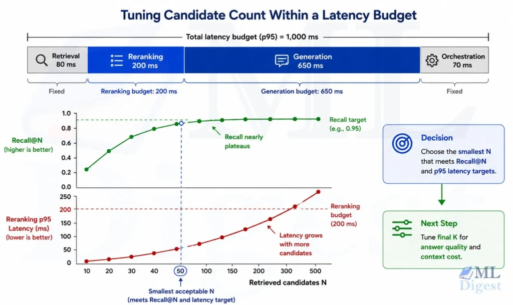
Measure the available time before selecting a model. If the total RAG budget is 1,000 ms and generation needs 650 ms, retrieval uses 80 ms, and orchestration uses 70 ms, the reranker has roughly 200 ms at the target percentile. This budget determines how many candidates can be cross-encoded and whether a larger reranker is feasible.
Benchmark the exact model, hardware, batch size, candidate count, and sequence length. Published throughput is not a substitute for measurement because truncation settings and payload lengths can dominate performance.
8.2 Tune $N$ before tuning $K$
Increase the retrieval candidate count $N$ until recall@$N$ is acceptable, then choose the smallest $N$ whose additional recall justifies reranking cost. Only afterward tune the final count $K$ against answer quality and context cost. Typical starting points are $N=50$, $K=5$ for cross-encoder RAG, but no universal setting exists.
8.3 Use hard negatives from your domain
Generic rerankers are strong baselines. Fine-tuning becomes worthwhile when rankings consistently fail on domain-specific distinctions, such as internal product names, legal exceptions, date validity, or document authority. Mine hard negatives from retrieved but non-clicked, non-cited, or annotator-rejected passages. Keep a clean validation split by query and document family to avoid leakage from near duplicates.
A relevance model may prefer an old but clearly worded policy over a newer authoritative version. Add metadata features or business rules for source authority, document date, access control, locale, and version. Evaluate version and effective-date metadata with point-in-time correctness in mind: the evidence must have been valid at the time the user asks about. Use these fields as explicit filters or carefully weighted features, rather than hoping the language model will infer every governance rule from prose.
8.5 Never skip safety evaluation
Retrieved content is untrusted input. Reranking can surface text that attempts to manipulate the generator, including instructions embedded in a document. Preserve source boundaries, instruct the generator to treat documents as data rather than commands, and scan or filter risky content as appropriate. See Guardrails for LLMs and Key Challenges for LLM Deployment for related controls.
9. Common failure modes
| Symptom | Likely cause | Practical response |
|---|---|---|
| Correct passage never reaches reranker | Candidate pool is too small or retrieval does not match the corpus language | Increase $N$, add hybrid retrieval, improve chunking, inspect recall@$N$ |
| Correct passage is present but ranked low | Generic reranker misses domain constraint | Inspect hard negatives, add metadata, fine-tune only after collecting labels |
| Results are redundant | Overlapping chunks dominate the top ranks | Deduplicate by source and span, then use MMR or a coverage rule |
| Good offline metric, poor answers | Generator receives too much context or lacks citation discipline | Tune $K$, require evidence-backed answers, evaluate answer support |
| Unpredictable latency | Candidate count or token lengths vary widely | Cap $N$ and sequence length, batch pairs, measure tail latency |
| Old policy wins | Relevance ignores freshness or authority | Filter by version, boost trusted sources, include validity metadata |
Summary
Reranking can improve RAG by separating broad recall from precise evidence selection. Bi-encoders retrieve quickly because they compare precomputed embeddings. Cross-encoders can make more precise pairwise judgments because query and passage tokens interact directly. Late-interaction models offer a useful middle ground when one vector is too coarse and full cross-encoding is too expensive.
A reasonable starting point is to compare a hybrid retriever with a dense-only baseline, retrieve around 50 candidates, cross-encode them, deduplicate the results, and pass three to five source-linked passages to the generator. Then evaluate the retrieval, ranking, and answer stages separately. The most useful next step is to build a small set of real queries, log the candidates before and after reranking, and measure whether the additional precision produces more supported answers within the latency budget.

Silpa brings 5 years of experience in working on diverse ML projects, specializing in designing end-to-end ML systems tailored for real-time applications. Her background in statistics (Bachelor of Technology) provides a strong foundation for her work in the field. Silpa is also the driving force behind the development of the content you find on this site.

Happy is a seasoned ML professional with over 15 years of experience. His expertise spans various domains, including Computer Vision, Natural Language Processing (NLP), and Time Series analysis. He holds a PhD in Machine Learning from IIT Kharagpur and has furthered his research with postdoctoral experience at INRIA-Sophia Antipolis, France. Happy has a proven track record of delivering impactful ML solutions to clients. Check more about him here: https://sites.google.com/site/slhappyin/
Subscribe to our newsletter!