Consider a bilingual dictionary. To understand a foreign word, you look it up and find its meaning. To express yourself in that language, you consult the same pages in reverse. One object, two directions.
A transformer language model works analogously. To read a token like “cat”, it retrieves a dense vector from an embedding table. To predict the next token, it scores every word in the vocabulary against the current hidden state. That scoring step is geometrically identical to the lookup: both compute similarity between a representation and each word’s stored vector.
Weight tying formalizes this symmetry. If reading and writing both measure the same kind of similarity in the same representational space, there is no principled reason for them to use separate matrices. Setting the output projection equal to the input embedding cuts the parameter count, regularizes the shared vector space, and consistently improves perplexity on language modeling benchmarks.
1. What Is Weight Tying?
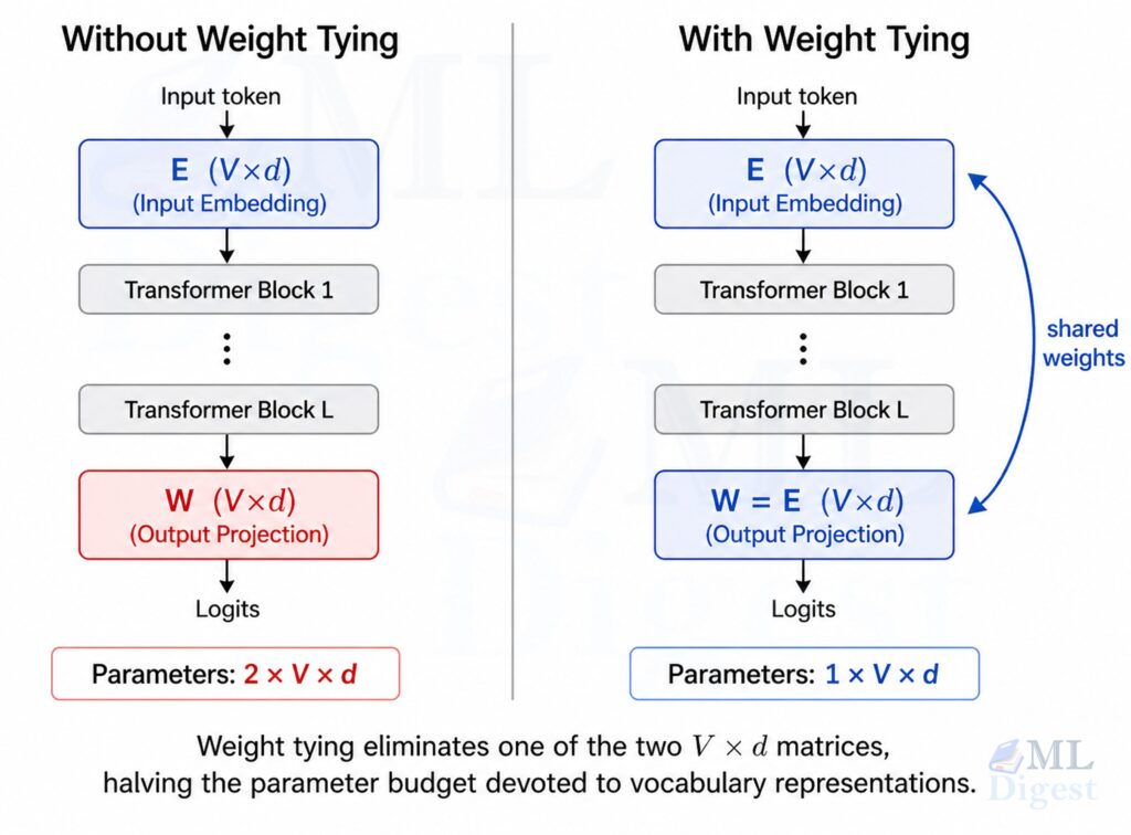
A standard transformer language model contains two large weight matrices that both involve the vocabulary:
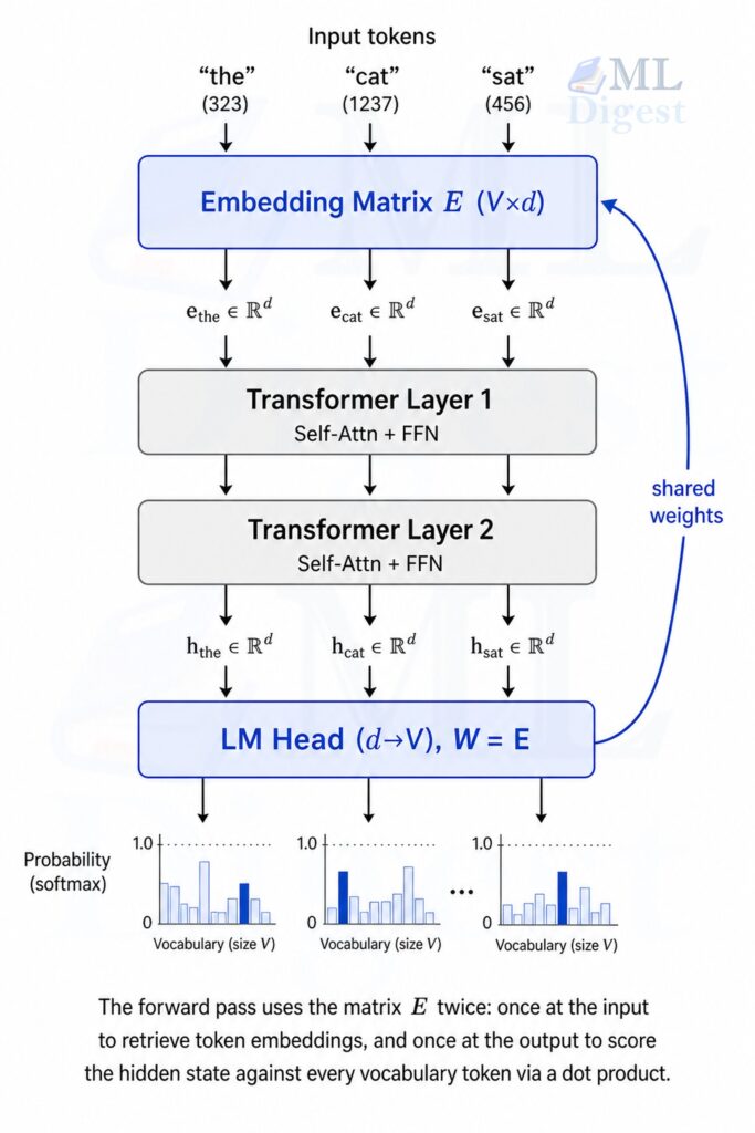
The input embedding matrix $E$ has shape $(V, d)$, where $V$ is the vocabulary size and $d$ is the model’s hidden dimension. Given a token index $i$, the model retrieves the row $E[i]$ as the token’s embedding vector.
The output projection matrix $W$ (the language model head) also has shape $(V, d)$. Given a final hidden state $\mathbf{h} \in \mathbb{R}^d$, the model computes $\text{logits} = \mathbf{h} W^\top$ to produce one score per vocabulary token.
Without weight tying, $E$ and $W$ are two independent matrices that each must be learned from scratch. With weight tying, we enforce $W = E$: a single matrix serves both roles simultaneously.
2. The Math
2.1 Forward Pass with Tied Weights
For a given token at position $t$, the transformer produces a hidden state $\mathbf{h}_t \in \mathbb{R}^d$ after the final layer. The unnormalized score (logit) for token $i$ being the next token is:
$$z_i = \mathbf{h}_t \cdot \mathbf{w}_i$$
where $\mathbf{w}_i$ is the $i$-th row of $W$. The probability distribution over the vocabulary is:
$$P(\text{token}_i \mid \text{context}) = \frac{e^{z_i}}{\sum_{j=1}^{V} e^{z_j}}$$
With weight tying, we set $\mathbf{w}_i = \mathbf{e}_i$ (the $i$-th row of the embedding matrix), so the logit becomes:
$$z_i = \mathbf{h}_t \cdot \mathbf{e}_i$$
This has a clean geometric interpretation: the model measures the dot product similarity between the final hidden state and each token’s embedding vector. The token whose embedding is most aligned with the hidden state is predicted as the most likely next token.
This is not merely a parameter-sharing trick. It enforces representational consistency: the geometry of the embedding space used to encode input meaning is the same geometry used to decode output predictions.
2.2 Parameter Savings
For a model with vocabulary size $V$ and hidden dimension $d$, the number of parameters in one embedding matrix is $V \times d$. Without weight tying you pay this cost twice. With weight tying you pay it once.
For GPT-2 small ($V = 50257$, $d = 768$):
$$50{,}257 \times 768 \approx 38.6 \text{ million parameters saved}$$
That is roughly 30% of GPT-2 small’s total parameter count recovered from a single architectural decision.
2.3 A Regularization Perspective
A less obvious benefit is implicit regularization. When the same matrix $E$ participates in both the embedding lookup and the output scoring, gradient updates flow through both paths simultaneously. The embedding of a token must simultaneously be a good contextual representation (input side) and a good scoring template for prediction (output side). This dual constraint discourages overfitting to either role in isolation and encourages more generalizable representations.
Two groups independently proposed and formalized this idea around the same time: Press and Wolf (2017) in Using the Output Embedding to Improve Language Models and Inan et al. (2017) in Tying Word Vectors and Word Classifiers: A Loss Framework for Language Modeling. Both demonstrated consistent perplexity improvements across multiple benchmarks with no increase in model size.
3. Implementation in PyTorch
The following is a minimal but complete transformer language model with weight tying. Every component is annotated to connect back to the theory above.
import torch
import torch.nn as nn

class TransformerLM(nn.Module):
    """
    A minimal causal Transformer language model with weight tying.

    The input embedding matrix and the output projection share the same
    weights, as introduced by Press & Wolf (2017).
    """

    def __init__(
        self,
        vocab_size: int,
        embed_dim: int,
        num_heads: int,
        num_layers: int,
        max_seq_len: int,
        dropout: float = 0.1,
    ):
        super().__init__()

        # Input token embedding: maps integer token IDs to vectors of shape (embed_dim,)
        # Weight shape: (vocab_size, embed_dim)
        self.token_embedding = nn.Embedding(vocab_size, embed_dim)

        # Learned positional embedding: one vector per position in the sequence
        self.pos_embedding = nn.Embedding(max_seq_len, embed_dim)

        # Causal transformer encoder stack (used here as a decoder-style LM)
        encoder_layer = nn.TransformerEncoderLayer(
            d_model=embed_dim,
            nhead=num_heads,
            dim_feedforward=embed_dim * 4,
            dropout=dropout,
            batch_first=True,
        )
        self.transformer = nn.TransformerEncoder(encoder_layer, num_layers=num_layers)

        # Output projection: maps hidden states of shape (embed_dim,) to
        # per-token logits of shape (vocab_size,).
        # Weight shape: (vocab_size, embed_dim) -- same as the embedding matrix.
        # bias=False is required for weight tying because nn.Embedding has no bias.
        self.lm_head = nn.Linear(embed_dim, vocab_size, bias=False)

        # --- Weight tying ---
        # This is not a copy. Both attributes now reference the exact same tensor.
        # Any gradient update to one is automatically reflected in the other.
        self.lm_head.weight = self.token_embedding.weight

        self._init_weights()

    def _init_weights(self):
        # Initialize with a small normal distribution.
        # Because of weight tying, this also initializes lm_head.weight.
        nn.init.normal_(self.token_embedding.weight, mean=0.0, std=0.02)

    def forward(self, token_ids: torch.Tensor) -> torch.Tensor:
        """
        Args:
            token_ids: (batch_size, seq_len) integer token IDs.

        Returns:
            logits: (batch_size, seq_len, vocab_size) unnormalized scores.
        """
        batch_size, seq_len = token_ids.shape
        positions = torch.arange(seq_len, device=token_ids.device).unsqueeze(0)

        # Combine token and position representations
        x = self.token_embedding(token_ids) + self.pos_embedding(positions)

        # Causal mask: position t can only attend to positions 0 through t
        causal_mask = nn.Transformer.generate_square_subsequent_mask(
            seq_len, device=token_ids.device
        )
        x = self.transformer(x, mask=causal_mask, is_causal=True)

        # Project to vocabulary logits using the tied embedding matrix.
        # Internally: logits = x @ E^T, so logit_i = h · e_i (dot product)
        logits = self.lm_head(x)
        return logits

# ---------------------------------------------------------------------------
# Sanity check: confirm the weights are truly the same object in memory
# ---------------------------------------------------------------------------
model = TransformerLM(
    vocab_size=1000,
    embed_dim=128,
    num_heads=4,
    num_layers=2,
    max_seq_len=64,
)

assert (
    model.lm_head.weight.data_ptr() == model.token_embedding.weight.data_ptr()
), "Weight tying failed: the two matrices are not the same object."

print("Weight tying confirmed.")
print(f"Embedding weight shape : {model.token_embedding.weight.shape}")
print(f"LM head weight shape   : {model.lm_head.weight.shape}")
print(f"Total parameters       : {sum(p.numel() for p in model.parameters()):,}")

# Expected output:
#     Weight tying confirmed.
#     Embedding weight shape : torch.Size([1000, 128])
#     LM head weight shape   : torch.Size([1000, 128])
# Total parameters : 532,736The single line that performs the tie is:
self.lm_head.weight = self.token_embedding.weightBoth names now point to the same underlying tensor storage. PyTorch’s autograd engine accumulates gradients from both the embedding path and the output projection path into this single tensor, so no custom gradient hooks are needed.
4. Weight Tying in Practice: Major Models
Weight tying is not a fringe technique. It is a widespread default across many well-known language models, though not a universal one.
GPT-2 ties its wte (word token embedding) with the language model head. BERT uses tied weights in its masked language modeling prediction head. T5 takes it further by tying embeddings across both encoder and decoder with the output projection (“three-way tying”).
Not all large models follow this convention. The LLaMA family explicitly keeps the input embedding and output projection as independent parameters (tie_word_embeddings=False in the model config). At larger model scales, the embedding matrices represent a smaller fraction of total parameters, so the savings from tying become less significant relative to the potential benefit of giving the input and output layers independent capacity.
The Hugging Face Transformers library applies weight tying by default through the tie_weights() method present in most PreTrainedModel subclasses.
5. Practical Tips and Best Practices
5.1 Scale the Embeddings at the Input
When weight tying is used, it is common to scale the embedding vectors before they enter the transformer. The original Transformer paper multiplies each embedding by $\sqrt{d}$:
$$\mathbf{x}_i = \sqrt{d} \cdot E[i]$$
The reason is about magnitude balance. The original Transformer uses sinusoidal positional encodings whose values lie in $[-1, 1]$. Token embeddings, when initialized with small values, would have much smaller magnitudes. Summing them directly would let the positional signal dominate the input representation. Multiplying by $\sqrt{d}$ amplifies the embedding vectors into the same numerical range as the positional encodings, ensuring both sources of information contribute meaningfully to the residual stream from the very first layer.
5.2 Always Set bias=False in the Output Layer
The dimensions only align if the output linear layer has no bias. In PyTorch, nn.Embedding(V, d).weight has shape (V, d), and nn.Linear(d, V, bias=False).weight also has shape (V, d). A bias term in the linear layer is not prohibited, but it is an extra degree of freedom that the embedding side does not have, which breaks the conceptual symmetry of the tie.
5.3 Gradients Are Summed from Both Paths
Because the tied matrix receives gradient contributions from both the embedding lookup (cross-entropy loss backpropagated through the output projection) and any embedding regularization (if used), the effective gradient for the shared matrix is the sum of both. PyTorch handles this automatically, but it is worth knowing when inspecting gradient norms or debugging unusual training dynamics.
5.4 When Not to Tie
Weight tying assumes the input and output vocabularies are identical. In practice, the vocabulary is typically constructed using subword tokenization methods such as Byte Pair Encoding (BPE). In encoder-decoder translation models with separate source and target vocabularies, tying the encoder embeddings with the decoder output projection would be a category error. However, many multilingual models do share a joint vocabulary across languages, in which case tying is perfectly applicable even in an encoder-decoder setting.
There is also a scale argument. For very large models, the embedding matrix becomes a relatively small fraction of total parameters. In that regime, the parameter savings from tying are marginal, and keeping the two matrices independent allows the model to learn specialized input representations and output scoring templates. This is the rationale behind the LLaMA family’s decision to forgo weight tying.
6. Summary
Weight tying is one of those rare ideas that appear almost trivially obvious in hindsight yet deliver real, measurable value. By recognizing that embedding a token and scoring a token are geometrically identical operations (a dot product against the same vocabulary vectors), we can collapse two independent matrices into one. The result is fewer parameters, implicit regularization from the dual gradient signal, and training stability from the reduced parameter space, all without any decrease in model quality.
The core equation is simply:
$$z_i = \mathbf{h} \cdot \mathbf{e}_i$$
The hidden state is compared against every token embedding directly. The token whose embedding is most similar wins. The dictionary you read from at the input is the same dictionary you write with at the output.

Silpa brings 5 years of experience in working on diverse ML projects, specializing in designing end-to-end ML systems tailored for real-time applications. Her background in statistics (Bachelor of Technology) provides a strong foundation for her work in the field. Silpa is also the driving force behind the development of the content you find on this site.
Subscribe to our newsletter!