Imagine walking into a library where every book has a helpful librarian attached to it. If you ask about a topic like “language models,” the librarian points to the words that best distinguish one book from thousands of others. Common words such as “the” or “is” are ignored because they appear everywhere. Specific words such as “tokenization,” “retrieval,” or “embedding” matter more because they tell you what makes that document special. TF-IDF is that librarian in mathematical form.
Term Frequency-Inverse Document Frequency (TF-IDF) is one of the foundational weighting schemes in information retrieval, text mining, and classical natural language processing. Even in a world dominated by transformers and dense embeddings, TF-IDF remains useful because it is transparent, fast, surprisingly strong for lexical matching, and often the simplest baseline you should build first.
Let’s dive in!
1. Why TF-IDF matters
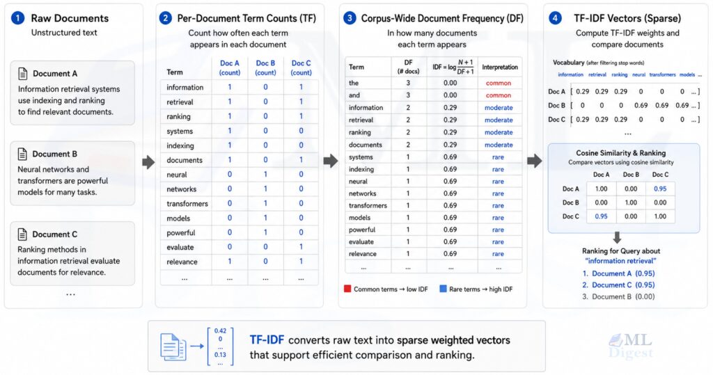
TF-IDF turns raw text into weighted numerical features. That sounds modest, but it solves a real problem.
If you only count words, then very common terms dominate the representation. A document with many occurrences of “the” is not more informative than one with fewer. TF-IDF adjusts for this by combining two signals:
- Term frequency (TF): how important a word is inside one document.
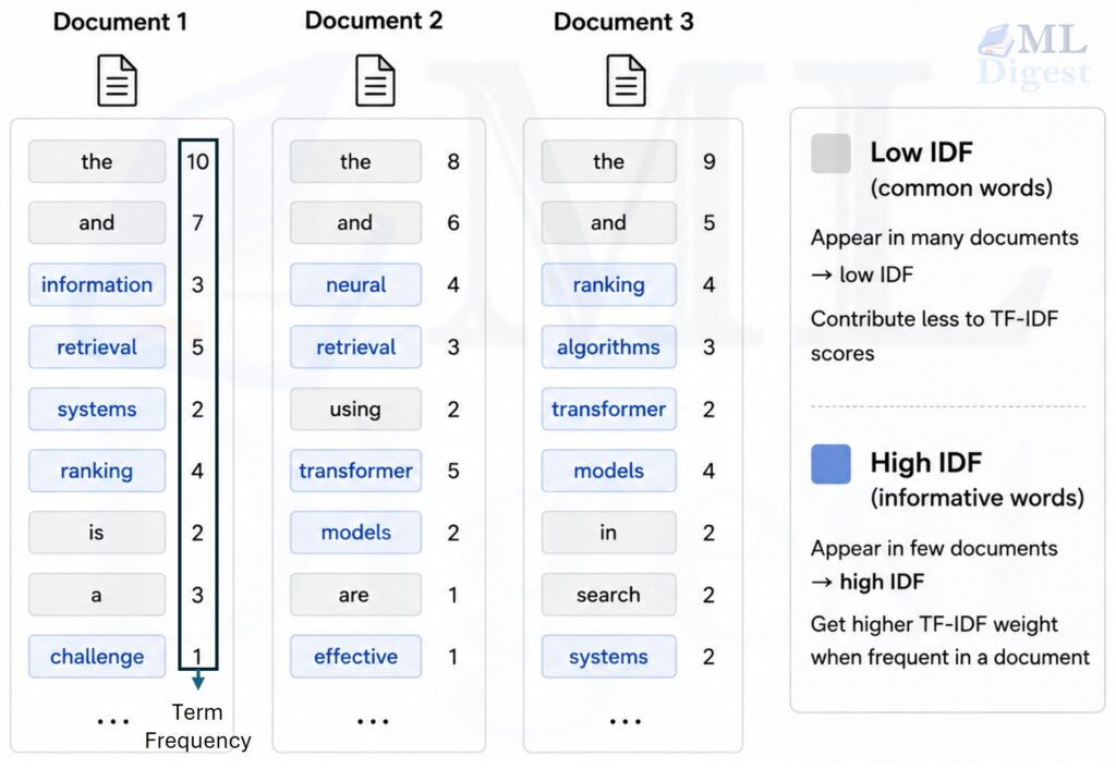
- Inverse document frequency (IDF): how rare and therefore informative the word is across the corpus.
This makes TF-IDF useful for tasks such as:
- document search and ranking
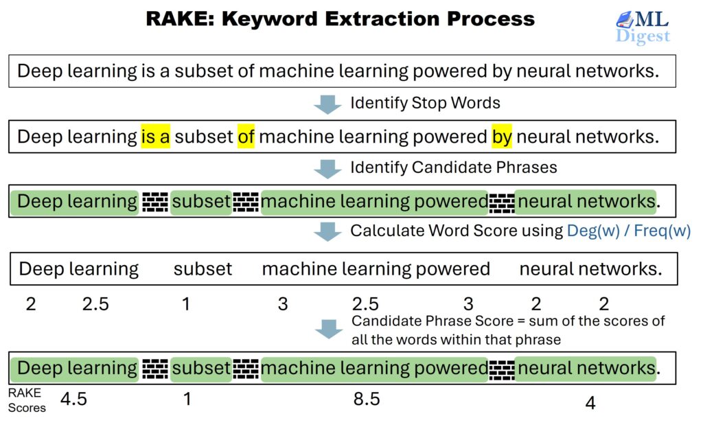
- keyword extraction
- document clustering
- spam filtering and text classification
- duplicate detection with cosine similarity
You will still see TF-IDF in production search stacks, feature engineering pipelines, and retrieval baselines because it is easy to debug and cheap to compute compared with neural representations.
2. The intuition behind the weighting
2.1 What plain term counts miss
Suppose you have two documents:
- “cats chase lasers in the living room”
- “dogs chase balls in the park”
If you represent both documents with plain bag-of-words counts, then words like “in” and “the” still take up space in the feature vector even though they barely help distinguish the documents.
The main idea behind TF-IDF is simple:
- A term should matter more if it appears many times in one document.
- A term should matter less if it appears in almost every document.
That balance is the core of TF-IDF.
2.2 A useful mental model
You can think of TF as local importance and IDF as global surprise.
- TF asks, “How loudly is this word speaking inside this document?”
- IDF asks, “How unusual is this word in the entire collection?”
TF-IDF multiplies those two ideas. A word gets a high score only when it is locally loud and globally unusual.
3. The mathematics of TF-IDF
3.1 Term frequency (TF)
For a term $t$ in document $d$, the simplest term frequency is just the raw count:
$$
\mathrm{tf}(t, d) = f_{t,d}
$$
where $f_{t,d}$ is the number of times term $t$ appears in document $d$.
In practice, several variants are common because raw counts can over-reward repeated words:
$$
\mathrm{tf}(t, d) = \frac{f_{t,d}}{\sum_{t’} f_{t’,d}}
$$
This normalized version divides by the document length.
Another common choice is sublinear scaling:
$$
\mathrm{tf}(t, d) =
\begin{cases}
1 + \log f_{t,d}, & f_{t,d} > 0 \
0, & f_{t,d} = 0
\end{cases}
$$
Sublinear TF is often a good practical default because the difference between 1 and 5 occurrences usually matters more than the difference between 101 and 105.
In practice, many libraries begin with count-based term frequencies and then apply IDF weighting plus a final normalization step. That is one reason raw counts often work well as a starting point even when the conceptual discussion begins with normalized TF.
3.2 Inverse document frequency (IDF)
Let $N$ be the number of documents in the corpus, and let $\mathrm{df}(t)$ be the number of documents that contain term $t$. The classic inverse document frequency is:
$$
\mathrm{idf}(t) = \log \frac{N}{\mathrm{df}(t)}
$$
The behavior is intuitive:
- If a term appears in many documents, then $\mathrm{df}(t)$ is large and IDF becomes small.
- If a term appears in only a few documents, then $\mathrm{df}(t)$ is small and IDF becomes large.
Many libraries use a smoothed version to avoid division by zero and make edge cases more stable. For example, scikit-learn’s TfidfVectorizer uses:
$$
\mathrm{idf}(t) = \log\left(\frac{1 + N}{1 + \mathrm{df}(t)}\right) + 1
$$
The smoothing serves two purposes:
- it avoids awkward edge cases in the ratio
- the final $+1$ keeps the weight positive instead of letting very common terms collapse to exact zero
3.3 The final TF-IDF weight
The final weight is the product:
$$
\mathrm{tfidf}(t, d) = \mathrm{tf}(t, d) \cdot \mathrm{idf}(t)
$$
This equation is simple, but it encodes the whole idea:
- repeated within the document
- uncommon across the corpus
That combination makes a term discriminative.
3.4 A small numeric example
Consider a corpus of $N = 3$ documents:
- “cat sat on mat”
- “cat ate fish”
- “dog ate fish”
For the term “cat”:
- $f_{\text{cat}, d_1} = 1$
- $\mathrm{df}(\text{cat}) = 2$
Using unsmoothed IDF:
$$
\mathrm{idf}(\text{cat}) = \log \frac{3}{2}
$$
For the term “mat”:
- $f_{\text{mat}, d_1} = 1$
- $\mathrm{df}(\text{mat}) = 1$
So:
$$
\mathrm{idf}(\text{mat}) = \log \frac{3}{1} = \log 3
$$
Since $\log 3 > \log(3/2)$, the term “mat” receives a larger TF-IDF weight than “cat” in document 1. That matches intuition because “mat” is more distinctive in this corpus.
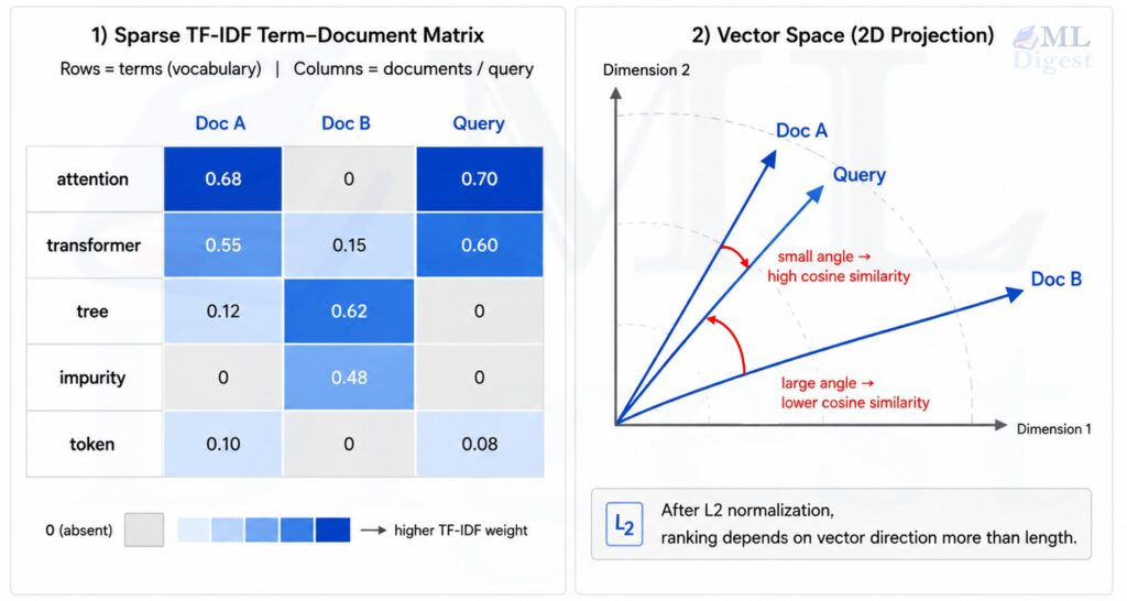
4. From weighted words to vector space
TF-IDF is usually paired with the vector space model, where each document is represented as a high-dimensional vector over the vocabulary.
If the vocabulary has $V$ unique terms, then document $d$ becomes:
$$
\mathbf{x}^{(d)} \in \mathbb{R}^{V}
$$
where each coordinate stores the TF-IDF weight of one term.
This representation lets you compare documents numerically. The most common similarity measure is cosine similarity:
$$
\cos(\theta) = \frac{\mathbf{x}^\top \mathbf{y}}{\lVert \mathbf{x} \rVert_2 \lVert \mathbf{y} \rVert_2}
$$
Cosine similarity focuses on direction rather than raw magnitude. That matters because two documents can discuss the same topic even if one is much longer than the other.
If the vectors are already $L_2$-normalized, cosine similarity reduces to a plain dot product. That is one reason normalized TF-IDF works so well in retrieval systems and linear models.
5. How TF-IDF is computed in practice
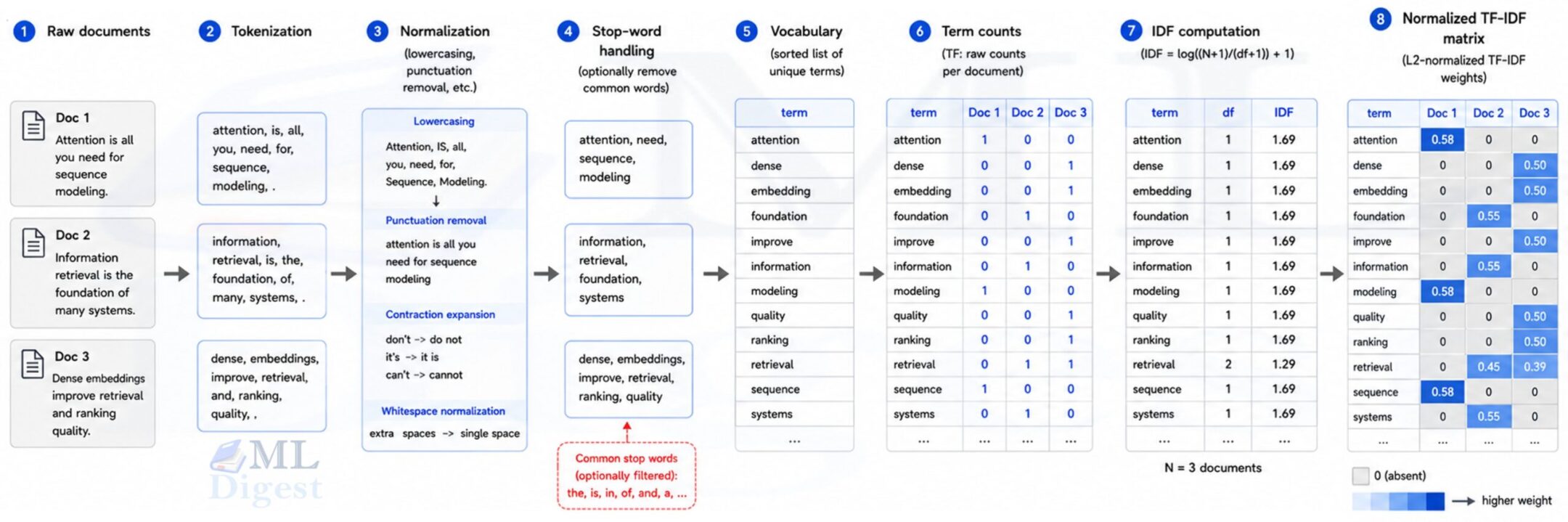
5.1 Typical pipeline
A standard TF-IDF pipeline looks like this:
- tokenize text into terms
- normalize text (for example, lowercase or Unicode normalization)
- optionally remove stop words
- build the vocabulary
- count term frequencies per document
- compute document frequencies across the corpus
- compute IDF values
- multiply TF by IDF
- optionally apply vector normalization such as $L_2$
The last step is important for retrieval and classification because normalization reduces document-length bias.
5.2 Tokenization choices matter
TF-IDF is conceptually simple, but the preprocessing choices strongly affect quality:
- word-level tokenization is the default for many tasks
- character n-grams can work well for noisy text, spelling variation, or multilingual search
- subword tokenization schemes such as byte pair encoding (BPE), WordPiece, and SentencePiece are worth considering when TF-IDF is part of a larger hybrid pipeline that also includes transformer-based components, since consistent tokenization can simplify feature alignment across retrieval stages
- stemming or lemmatization can reduce sparsity, but can also remove useful distinctions
- domain-specific stop-word lists often outperform generic ones
One lesson from practice is that most TF-IDF performance gains come from good tokenization and normalization choices, not from tweaking the formula endlessly.
6. A runnable Python example
The fastest way to understand TF-IDF is to compute it on a tiny corpus and inspect the weights.
from sklearn.feature_extraction.text import TfidfVectorizer
from sklearn.metrics.pairwise import cosine_similarity

documents = [
    "transformers use attention mechanisms for sequence modeling",
    "attention helps transformers focus on relevant tokens",
    "decision trees split features using impurity measures",
]

query = ["attention in transformer models"]

vectorizer = TfidfVectorizer(
    lowercase=True,
    stop_words="english",
    ngram_range=(1, 2),
    sublinear_tf=True,
    smooth_idf=True,
    norm="l2",
)

doc_matrix = vectorizer.fit_transform(documents)
query_vector = vectorizer.transform(query)

scores = cosine_similarity(query_vector, doc_matrix).ravel()

feature_names = vectorizer.get_feature_names_out()
first_doc_dense = doc_matrix[0].toarray().ravel()
top_indices = first_doc_dense.argsort()[::-1][:8]

print("Top weighted terms in document 1:")
for index in top_indices:
    if first_doc_dense[index] > 0:
        print(f"{feature_names[index]:<25} {first_doc_dense[index]:.3f}")

print("\nQuery-to-document cosine similarities:")
for doc_id, score in enumerate(scores, start=1):
print(f"Document {doc_id}: {score:.3f}")What this example demonstrates:
fit_transformlearns the vocabulary and IDF values from the corpustransformapplies the same mapping to new text such as a query- cosine similarity ranks documents by lexical overlap after TF-IDF weighting
- bigrams such as
attention mechanismscan become useful features whenngram_range=(1, 2)
If you run this example, the two transformer-related documents should score higher than the decision-tree document. That is exactly the kind of lightweight lexical retrieval baseline TF-IDF is good at.
6.1 A minimal NumPy-style implementation
It is also useful to see the core logic without a library wrapper.
import math
from collections import Counter

documents = [
    ["cat", "sat", "on", "mat"],
    ["cat", "ate", "fish"],
    ["dog", "ate", "fish"],
]

vocabulary = sorted({token for doc in documents for token in doc})
doc_count = len(documents)

document_frequency = {}
for term in vocabulary:
    document_frequency[term] = sum(term in set(doc) for doc in documents)

idf = {
    term: math.log((1 + doc_count) / (1 + document_frequency[term])) + 1
    for term in vocabulary
}

tfidf_vectors = []
for doc in documents:
    counts = Counter(doc)
    doc_length = len(doc)
    vector = {}
    for term, count in counts.items():
        tf = count / doc_length
        vector[term] = tf * idf[term]
    tfidf_vectors.append(vector)

for doc_id, vector in enumerate(tfidf_vectors, start=1):
print(f"Document {doc_id}: {vector}")This version makes the mechanics explicit:
- count terms per document
- count how many documents contain each term
- compute IDF once for the corpus
- multiply normalized TF by IDF
6.2 A classification pipeline in scikit-learn
TF-IDF is not only for retrieval. It is also a strong feature representation for supervised text classification.
from sklearn.feature_extraction.text import TfidfVectorizer
from sklearn.linear_model import LogisticRegression
from sklearn.pipeline import Pipeline

model = Pipeline(
    [
        (
            "tfidf",
            TfidfVectorizer(
                ngram_range=(1, 2),
                min_df=2,
                max_df=0.95,
                sublinear_tf=True,
                norm="l2",
            ),
        ),
        ("clf", LogisticRegression(max_iter=2000)),
    ]
)

# model.fit(train_texts, train_labels)
# predictions = model.predict(test_texts)This pattern matters because the same fitted vectorizer must be reused at inference time. If you rebuild the vocabulary separately for training and prediction, the feature dimensions no longer line up.
7. Practical considerations for real-world use
- Choose normalization deliberately:
If your downstream task uses cosine similarity or linear models, $L_2$ normalization is often a sensible default. Without it, long documents may dominate simply because they contain more tokens. - Use n-grams when phrases carry meaning:
Unigrams are often enough for simple tasks, but phrases such as “machine learning,” “credit risk,” or “customer churn” carry meaning that single tokens miss. Adding bigrams often produces a noticeable improvement. - Be careful with stop-word removal:
Removing stop words is common, but it is not always correct. In sentiment analysis, for example, words such as “not” can carry essential meaning. Always validate preprocessing choices against the task. - Prefer sparse matrices for real corpora:
TF-IDF vectors are usually extremely sparse. Use sparse matrix representations from SciPy or libraries built on top of it. Converting a large TF-IDF matrix to a dense array is a common beginner mistake and can waste a large amount of memory. - Sublinear TF is often a good default:
Repeated mentions do matter, but not linearly forever. If one document repeats a word 50 times, it is not necessarily 50 times more about that concept than a document that mentions it twice. - Fit on training data only:
In machine learning workflows, IDF is part of the learned representation because it depends on corpus-wide statistics. That means you should fit the vectorizer on the training split only, then use the fitted vectorizer to transform validation, test, and production inputs.
If you fit TF-IDF on the full dataset before splitting, you leak information from the evaluation set into the representation. The effect is subtle, but it can make offline metrics look better than the real system deserves. - Control vocabulary growth:
Large vocabularies can hurt memory usage, training speed, and generalization. In practice, a few parameters matter a lot:min_dfremoves extremely rare terms that often behave like noisemax_dfremoves overly common terms that add little signalmax_featurescaps dimensionality when the corpus is very large
- Reuse the same vectorizer at inference time:
TF-IDF vectors are only comparable when they come from the same vocabulary, IDF statistics, and preprocessing pipeline. Save the fitted vectorizer and reuse it exactly as-is for later queries, classification requests, or similarity comparisons.
This avoids feature misalignment, vocabulary drift, and inconsistent behavior between training and deployment.
8. Best practices for common tasks
8.1 Document retrieval
For search, TF-IDF is a strong lexical baseline. It works especially well when exact terms matter, such as product names, code identifiers, legal phrases, or medical terminology.
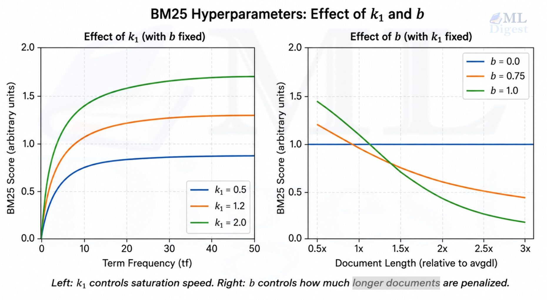
If you need stronger ranking, TF-IDF is often followed by BM25, which adjusts term saturation and document-length effects more explicitly.
8.2 Text classification
TF-IDF paired with logistic regression or linear support vector machines is still a very competitive baseline for many text classification tasks. Before building a larger neural model, it is often worth checking whether a linear classifier on TF-IDF already solves most of the problem.
8.3 Clustering and exploration
For clustering or exploratory analysis, TF-IDF can help surface topical structure, especially when combined with dimensionality reduction. A standard approach is to apply truncated singular value decomposition (SVD) to the TF-IDF matrix, which is the foundation of Latent Semantic Analysis (LSA). LSA compresses the sparse high-dimensional representation into a dense lower-dimensional space that captures latent topic structure, often producing more stable clusters than raw TF-IDF vectors. However, high-dimensional sparsity can still make clustering noisy before this step, so preprocessing and feature pruning remain important.
9. Limitations and failure modes
TF-IDF is useful, but it has clear limits.
- No semantic understanding:
TF-IDF is lexical. It only knows which tokens appear, not what they mean. It does not know that “car” and “automobile” are related unless both appear in similar patterns or you engineer features for that.
If you need some degree of semantic generalization without the cost of transformer models, fastText represents a useful middle step. Rather than assigning purely corpus-specific term weights, fastText learns subword-level distributed representations that can generalize across surface forms and handle out-of-vocabulary words, two properties that TF-IDF lacks by design. - Sensitive to vocabulary mismatch:
If a query uses different wording from a document, TF-IDF may miss the match. Dense retrieval methods and transformer embeddings handle this semantic gap better. - Sparse and high-dimensional:
The vectors can become very large when the vocabulary explodes. This is manageable with sparse matrices, but feature pruning is often necessary. - Corpus-dependent weights:
IDF values depend on the corpus. If the document collection changes substantially, you may need to refit the vectorizer so the weights still reflect the new distribution.
10. TF-IDF versus modern embedding methods
It is tempting to think of TF-IDF as obsolete, but that is not the right framing.
TF-IDF and embeddings solve different problems well:
- TF-IDF is precise for lexical overlap, transparent, and fast.
- Embeddings are better for semantic matching, paraphrases, and broader generalization.
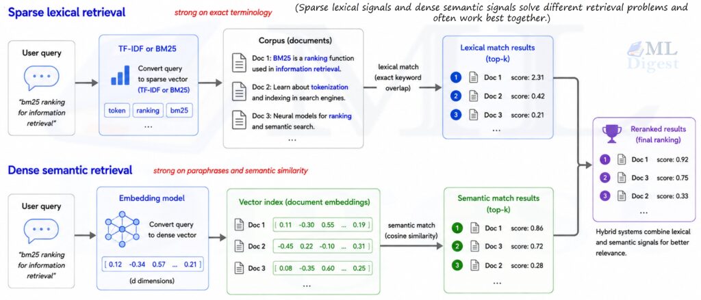
In many real systems, both are useful. A retrieval stack may use TF-IDF or BM25 for initial sparse retrieval and then rerank with neural models. In other settings, TF-IDF is simply the right tool because explainability, latency, or data scarcity matter more than semantic sophistication.
The same hybrid pattern shows up in retrieval-augmented generation (RAG), where sparse lexical retrieval and dense semantic retrieval often complement each other.
Summary
TF-IDF remains one of the clearest examples of how a simple idea can become a durable engineering tool. It rewards terms that are frequent in one document and rare across the corpus, producing interpretable sparse vectors that work well for retrieval, classification, and exploration.
If you want to go further, a sensible sequence is: implement TF-IDF from scratch once, compare it with scikit-learn’s TfidfVectorizer, then study Introduction to Information Retrieval and BM25 to understand how classical ranking systems improve on the same core intuition.

Silpa brings 5 years of experience in working on diverse ML projects, specializing in designing end-to-end ML systems tailored for real-time applications. Her background in statistics (Bachelor of Technology) provides a strong foundation for her work in the field. Silpa is also the driving force behind the development of the content you find on this site.

Happy is a seasoned ML professional with over 15 years of experience. His expertise spans various domains, including Computer Vision, Natural Language Processing (NLP), and Time Series analysis. He holds a PhD in Machine Learning from IIT Kharagpur and has furthered his research with postdoctoral experience at INRIA-Sophia Antipolis, France. Happy has a proven track record of delivering impactful ML solutions to clients.
Subscribe to our newsletter!