Detection Transformers (DETR) Made Easy: End-to-End Object Detection with Transformers

Paper: End-to-End Object Detection with Transformers (Carion et al., 2020)

Imagine you are a detective assigned to a crime scene. The classic approach is to first carpet the entire room with 1,000 numbered placards, one on every spot where a clue might be, then go back and remove the redundant ones. That is essentially what anchor-based detectors do: blanket the image with candidate boxes and then prune.

Now imagine a different detective who walks in with exactly 100 folders, hands each folder to a different colleague, and says “you are responsible for finding one specific thing in this room.” Each colleague scans the whole scene, coordinates with the others to avoid doubling up, and fills in their folder or marks it “nothing found.” No redundant placards, no post-processing sweep. That is the spirit of DETR.

DETR (DEtection TRansformer) recasts object detection as a direct set prediction problem and uses a Transformer encoder-decoder to solve it. No anchors. No non-maximum suppression. One loss. One model.

1. The Problem with Classic Detectors

To appreciate why DETR matters, it helps to understand what it is replacing.

Methods like Faster R-CNN and RetinaNet produce detections through a pipeline assembled from several hand-designed stages:

• A dense anchor grid defines thousands of candidate boxes at fixed scales and aspect ratios across the image.
• A network classifies each anchor and refines its coordinates.
• Non-maximum suppression (NMS) removes duplicate predictions that overlap beyond a threshold.

These components work well, but they introduce geometry-specific inductive biases that must be tuned per dataset. More importantly, they make the pipeline non-end-to-end in a strict sense: the NMS step is not differentiable, and the anchor design requires domain expertise.

DETR asks: what if the network itself learned to produce exactly the right detections, without any post-processing?

2. Detection as Set Prediction

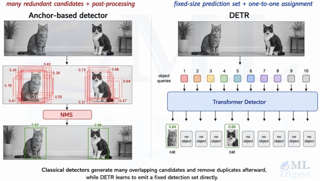
The core idea of DETR is elegantly simple. Given an image, produce a fixed-size set of $N$ predictions. Each prediction is either a detected object (with class and bounding box) or “nothing here.”

A concrete illustration. As shown in the above figure, an image contains two cats.

• A classic detector (YOLO or Faster R-CNN) might output five boxes around the first cat and three around the second, all with high confidence. NMS is then called to delete the six duplicate boxes based on overlap.
• DETR outputs exactly 100 predictions. It is trained so that if slot 5 predicts Cat A, slot 42 must not also predict Cat A. The network resolves the conflict internally, not in a post-processing step.

This is only possible because of a clever training objective: Hungarian matching (covered in detail). During training, each ground-truth object is assigned to exactly one prediction slot, and the model is penalized for any other slot that tries to claim the same object.

What changes compared to anchor-based detectors:

• There are no hand-designed anchor priors.
• There is no NMS stage at inference.
• A single loss supervises the whole pipeline end-to-end.

3. Architecture Overview

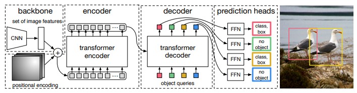
The pipeline in four steps:

1. Backbone. An image $(x_{img}\in\mathbb{R}^{3\times H_0 \times W_0 })$ enters a ResNet (ResNet-50 or ResNet-101) and is compressed into a feature map with $C=2048$ channels at spatial resolution $H \times W$, where $H = H_0 / 32$ and $W = W_0 / 32$. The value of $H$ and $W$ depends on the input image size, but the spatial downsampling by a factor of 32 is fixed.
2. Transformer Encoder. First a 1×1 convolution reduces the channel dimension from $C=2048$ to $d=256$, creating a feature map of dimension $d \times H \times W$. This feature map is then flattened into a sequence of $H \cdot W$ tokens, augmented with 2D positional encodings, and passed through encoder layers. Every spatial token can attend to every other token, building global context.
3. Transformer Decoder. $N$ learned object query embeddings enter the decoder. Each query self-attends with other queries, then cross-attends to the encoder output. The result is $N$ output embeddings, one per detection slot.
4. Prediction Heads. Each output embedding passes through a linear layer (class logits) and a 3-layer MLP (bounding box coordinates), producing $N$ class-box pairs.

3.1 Backbone and feature projection

The backbone output is:

$$\mathbf{F} \in \mathbb{R}^{C \times H \times W}$$

A $1 \times 1$ convolution projects it from $C$ channels to the Transformer model dimension $d$:

$$\mathbf{X} \in \mathbb{R}^{d \times H \times W}$$

Spatially flattened and transposed to sequence-first format, the encoder input is:

$$\mathbf{X} \in \mathbb{R}^{(HW) \times d}$$

3.2 2D Positional Encodings

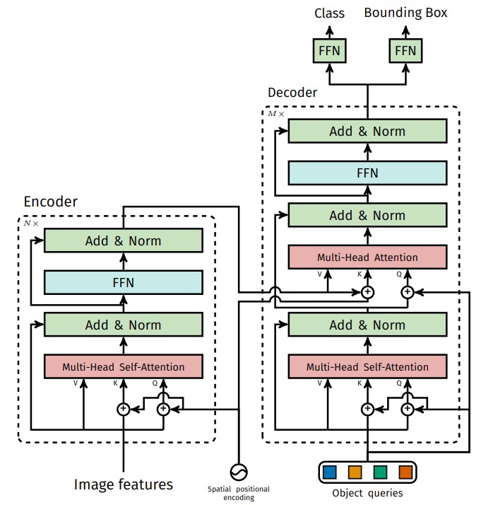
Self-attention is permutation-equivariant: it does not attach any meaning to absolute token order on its own, so there is no inherent notion of “this token came from the top-left corner.” DETR injects spatial information by adding 2D positional encodings at the input of each attention layer within the encoder (not just once at the encoder input). The general motivation is the same as in absolute vs. relative position embeddings, even though DETR applies the idea over a 2D grid instead of a 1D token stream.

The paper uses sine-cosine encodings adapted to a 2D grid. For a spatial location $(u, v)$, the encoding is formed by concatenating the standard 1D sine-cosine encoding applied to $u$ (using half the dimensions) and the same applied to $v$ (using the other half):

$$\text{pos}(u, v) \in \mathbb{R}^{d}$$

At each encoder attention layer, $\text{pos}$ is added to both the queries and keys before the self-attention computation, while values use $\mathbf{X}$ without positional information.

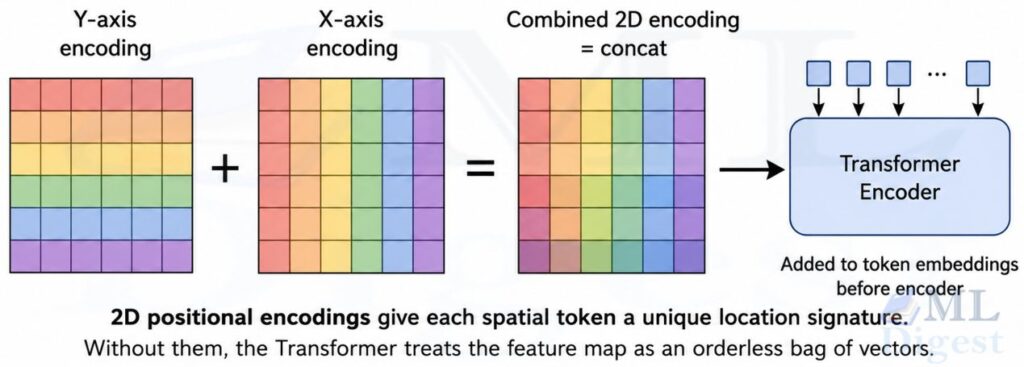
Without these encodings, the encoder would treat the feature map as a bag of vectors: a feature from the top-left corner would be indistinguishable from one at the bottom-right.

3.3 Transformer Encoder

The encoder is a standard stack of Transformer encoder layers. Each layer applies:

1. Multi-head self-attention over all $HW$ tokens.
2. A position-wise feed-forward network.
3. Residual connections and layer normalization.

The purpose is to enrich each spatial token with global context. Spatial regularities, long-range dependencies, and object-part relationships are captured here before any detection decision is made. If you want the attention primitive itself broken down separately, see attention mechanisms in Transformers and different attention variants in the taxonomy of attention mechanisms.

3.4 Transformer Decoder and Object Queries

The decoder takes $N$ learned vectors called object queries as input. These are not boxes and not region proposals.

These are not boxes or region proposals; they are fixed $d$-dimensional vectors (an embedding matrix or a set of learned parameters) that the model initializes (usually randomly) and learns end-to-end. The same $N$ query vectors are reused for every image (the paper uses $N=100$). They are model parameters, not outputs of the backbone. At runtime these learned queries are fed into the decoder.

Note that all the $N$ objects are decoded parallelly (independently) by the decoder (in contrast to an autoregressive decoder of original Transformers).

Each decoder layer performs:

1. Self-attention among the $N$ queries (so different slots coordinate and avoid predicting the same object).
2. Cross-attention from the queries to the encoder output (so each slot reads the relevant parts of the image); if you want a separate intuition for that operation, see cross-attention.
3. A position-wise feed-forward network.

After the final decoder layer, each of the $N$ query embeddings represents one candidate detection.

What do object queries actually learn?

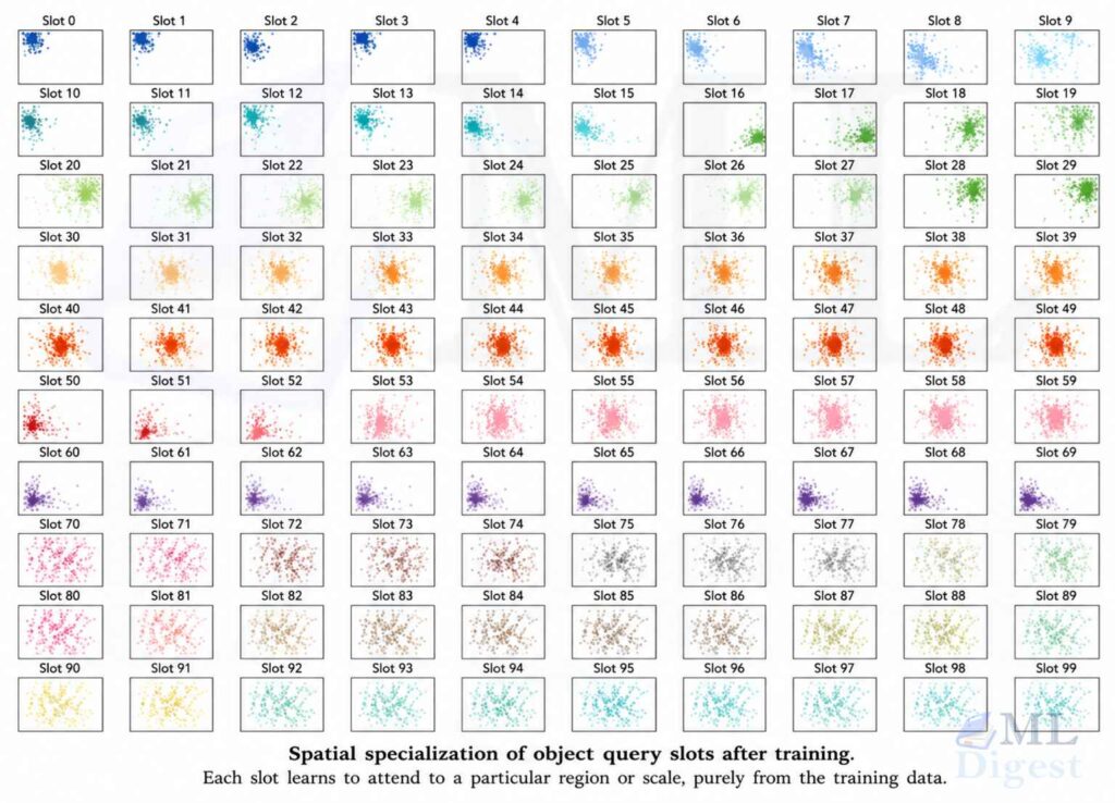
If you visualize the boxes predicted by each specific query slot across the validation set, a striking pattern emerges: the slots specialize spatially.

• Query index 35 might specialize in large, centrally located objects.
• Query index 60 might consistently look for objects in the bottom-left corner.
• Query index 90 might be a catch-all for small objects.

Unlike anchors in Faster R-CNN, which form rigid hand-designed grids, these specializations are learned entirely from data and adapt to the statistics of the training distribution.

3.5 Prediction Heads

For each query embedding $\mathbf{z}_i \in \mathbb{R}^{d}$:

• A linear layer predicts class logits over $K+1$ classes (the extra class is the “no object” class $\varnothing$).
• A 3-layer MLP predicts box coordinates $(c_x, c_y, w, h)$ relative to the image size in $[0,1]$, with a sigmoid applied to the output.

4. Problem Formulation

DETR outputs a fixed-size set of $N$ predictions:

$$\hat{y} = {\hat{y}_i}_{i=1}^{N}$$

Each prediction is a tuple:

$$\hat{y}_i = (\hat{p}_i,\, \hat{b}_i)$$

where $\hat{p}_i \in \mathbb{R}^{K+1}$ is a categorical distribution (computed by applying softmax to the class logits) over $K$ object classes plus a single “no-object” class: the extra class corresponds to the $(K+1)$-th softmax component. And $\hat{b}_i = (\hat{c}_x, \hat{c}_y, \hat{w}, \hat{h}) \in [0,1]^4$ is a normalized bounding box.

The ground truth for an image is a set of $M$ objects:

$$y = {y_j}_{j=1}^{M}, \quad y_j = (c_j,\, b_j)$$

Since $N$ is fixed (the paper uses $N=100$) and $M$ varies per image, the training objective must decide which of the $N$ predictions should match which of the $M$ ground-truth objects. This is the job of Hungarian matching.

5. The Training Objective: Hungarian Matching and Set Loss

This is the heart of DETR. Everything else is a standard Transformer on top of a standard backbone. What is genuinely novel is how the training loss is computed.

5.1 Why matching is needed

The $N$ output slots are symmetric: if query 7 predicts the dog and query 12 predicts the person, swapping them does not change the quality of the detection set. The loss must therefore first decide “which prediction is responsible for which ground-truth object” before it can penalize anything.

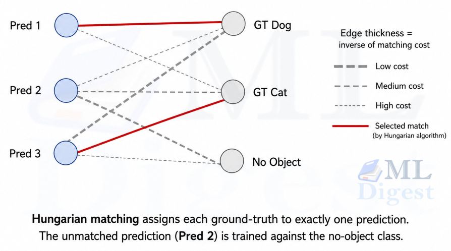
A simplified matching walkthrough. Suppose $N=3$ and there are $M=2$ ground-truth objects (a dog and a cat). The pairwise cost matrix might look like this:

The Hungarian algorithm finds the unique assignment that minimizes total cost. The best assignment is GT 1 to Pred 1 and GT 2 to Pred 3, with a total cost of $-0.8 + (-0.9) = -1.7$. Pred 2 is assigned the no-object class. Any other valid assignment yields a higher cost.

5.2 Hungarian (bipartite) matching

Formally, DETR solves a linear assignment problem. Let $\sigma$ be a permutation that maps each ground-truth index $j$ to a prediction index $\sigma(j)$. The optimal assignment is:

$$\hat{\sigma} = \arg\min_{\sigma} \sum_{j=1}^{M} \mathcal{C}(y_j,\, \hat{y}_{\sigma(j)})$$

The pairwise matching cost combines classification confidence and box quality:

$$\mathcal{C}(y_j,\, \hat{y}_i) = -\hat{p}_i(c_j) + \lambda_{\text{L1}} \lVert b_j – \hat{b}_i \rVert_1 + \lambda_{\text{giou}} \bigl(1 – \text{GIoU}(b_j,\, \hat{b}_i)\bigr)$$

Three terms are at work here:

• $-\hat{p}_i(c_j)$ encourages matching targets to predictions that are already confident about the correct class.
• The $\ell_1$ term measures the raw parameter-space distance between the target and predicted box.
• GIoU (Generalized IoU) extends standard IoU by subtracting a penalty proportional to the fraction of the smallest enclosing box not covered by either box: the “dead space” between them. This provides a non-zero gradient even when the two boxes have zero overlap, which plain IoU cannot.

The matching step is non-differentiable, but it only selects which pairs to compute losses on. Gradients flow through the loss terms on the matched pairs, not through the matching itself.

5.3 Set prediction loss

Once $\hat{\sigma}$ is fixed, the total set loss is:

$$\mathcal{L} = \sum_{j=1}^{M} \Bigl(\mathcal{L}_\text{cls}(c_j,\, \hat{p}_{\hat{\sigma}(j)}) + \mathcal{L}_\text{box}(b_j,\, \hat{b}_{\hat{\sigma}(j)})\Bigr) + \sum_{i \in \text{unmatched}} \mathcal{L}_\text{cls}(\varnothing,\, \hat{p}_i)$$

Matched predictions receive both a classification loss and a box regression loss. Unmatched predictions receive only a classification loss that pushes them toward the no-object class.

Classification loss. Cross-entropy over $K+1$ classes. Because most predictions are unmatched, the no-object class is down-weighted by a factor $\lambda_{\varnothing}$ (the paper uses $0.1$) to prevent the model from collapsing to predicting $\varnothing$ everywhere.

Box loss. For a matched pair:

$$\mathcal{L}_\text{box} = \lambda_{\text{L1}} \lVert b_j – \hat{b}_{\hat{\sigma}(j)} \rVert_1 + \lambda_{\text{giou}} \bigl(1 – \text{GIoU}(b_j,\, \hat{b}_{\hat{\sigma}(j)})\bigr)$$

The combination of $\ell_1$ and GIoU handles both scale-independent accuracy and the non-overlap regime.

Auxiliary decoding losses. In the original paper, the same classification and box heads are applied at the output of each intermediate decoder layer, and their losses are summed. In the official DETR training setup, Hungarian matching is computed for the final output and then recomputed for each auxiliary decoder output before that layer’s set loss is evaluated. This auxiliary supervision significantly improves optimization.

5.4 Results

At a high level, DETR with a ResNet-50 backbone matches the performance of a well-tuned Faster R-CNN on COCO while removing the anchor design and NMS entirely.

• Large objects. DETR excels here. The global receptive field of the Transformer lets each object query see the entire image at once, which is particularly advantageous for large objects that span a significant fraction of the scene.
• Small objects. The original DETR underperforms on small objects. Small objects map to very few pixels in the $H/32 \times W/32$ feature map, and without multi-scale features, the Transformer cannot attend to them efficiently.

For detailed AP numbers across scales, backbones, and training schedules, the original paper tables are the authoritative reference.

6. Inference: Why NMS is Not Needed

At inference time, the forward pass is simply:

1. Run the image through backbone, encoder, and decoder to obtain $N$ prediction pairs $(\hat{p}_i, \hat{b}_i)$.
2. For each prediction, take the argmax of $\hat{p}_i$. Discard predictions whose most likely class is $\varnothing$.
3. Optionally apply a confidence threshold or keep only the top-$k$ predictions.

Because the model is trained with one-to-one matching and query self-attention, two different slots rarely produce overlapping high-confidence detections for the same object. This is a sharp contrast with classical CNN-based detectors, which depend more heavily on localized receptive fields, proposal machinery, and post-processing. The one-to-one assignment pressure during training is what makes NMS unnecessary.

7. Implementation

import torch
import torch.nn as nn


class MLP(nn.Module):
    """Simple multi-layer perceptron used for the bounding box prediction head."""

    def __init__(self, input_dim: int, hidden_dim: int, output_dim: int, num_layers: int):
        super().__init__()
        layers = []
        for i in range(num_layers):
            in_dim = input_dim if i == 0 else hidden_dim
            out_dim = output_dim if i == num_layers - 1 else hidden_dim
            layers.append(nn.Linear(in_dim, out_dim))
            if i < num_layers - 1:
                layers.append(nn.ReLU())
        self.net = nn.Sequential(*layers)

    def forward(self, x: torch.Tensor) -> torch.Tensor:
        return self.net(x)


class DETR(nn.Module):
    """
    Minimal DETR model skeleton illustrating the data-flow and tensor shapes.

    backbone   -- returns (features [B,C,H,W], pos [B,d,H,W], mask [B,H,W])
    transformer -- standard PyTorch Transformer encoder-decoder
    num_classes -- number of object categories (no-object class added automatically)
    num_queries -- N, the fixed-size detection budget (paper: 100)
    d_model     -- Transformer hidden dimension (paper: 256)
    """

    def __init__(self, backbone, transformer, num_classes: int,
                 num_queries: int = 100, d_model: int = 256):
        super().__init__()
        self.backbone = backbone
        # Project backbone output channels to the Transformer dimension
        self.input_proj = nn.Conv2d(backbone.out_channels, d_model, kernel_size=1)
        self.transformer = transformer
        # N learned object query embeddings -- the detection slots
        self.query_embed = nn.Embedding(num_queries, d_model)

        self.class_head = nn.Linear(d_model, num_classes + 1)   # +1 for no-object
        self.bbox_head  = MLP(d_model, d_model, 4, num_layers=3)

    def forward(self, images: torch.Tensor):
        # features: [B, C, H, W]  -- backbone conv features
        # pos:      [B, d, H, W]  -- 2D sine-cosine positional encodings
        # mask:     [B, H, W]     -- padding mask (True where padded)
        features, pos, mask = self.backbone(images)

        src = self.input_proj(features)          # [B, d, H, W]
        B, d, H, W = src.shape

        # Flatten spatial dimensions; Transformer expects sequence-first
        src_flat  = src.flatten(2).permute(2, 0, 1)   # [HW, B, d]
        pos_flat  = pos.flatten(2).permute(2, 0, 1)   # [HW, B, d]
        mask_flat = mask.flatten(1)                    # [B, HW]

        # Repeat queries for each item in the batch
        query = self.query_embed.weight.unsqueeze(1).repeat(1, B, 1)  # [N, B, d]

        # hs: [L, N, B, d]  -- decoder outputs from each of L layers
        hs = self.transformer(src_flat, mask_flat, pos_flat, query)
        out = hs[-1]  # [N, B, d]  -- take the final decoder layer output

        logits = self.class_head(out)          # [N, B, K+1]
        boxes  = self.bbox_head(out).sigmoid() # [N, B, 4]  -- values in [0, 1]

        # Return batch-first tensors
        return logits.permute(1, 0, 2), boxes.permute(1, 0, 2)
        # logits: [B, N, K+1]
        # boxes:  [B, N, 4]

import torch
import torch.nn as nn


class MLP(nn.Module):
    """Simple multi-layer perceptron used for the bounding box prediction head."""

    def __init__(self, input_dim: int, hidden_dim: int, output_dim: int, num_layers: int):
        super().__init__()
        layers = []
        for i in range(num_layers):
            in_dim = input_dim if i == 0 else hidden_dim
            out_dim = output_dim if i == num_layers - 1 else hidden_dim
            layers.append(nn.Linear(in_dim, out_dim))
            if i < num_layers - 1:
                layers.append(nn.ReLU())
        self.net = nn.Sequential(*layers)

    def forward(self, x: torch.Tensor) -> torch.Tensor:
        return self.net(x)


class DETR(nn.Module):
    """
    Minimal DETR model skeleton illustrating the data-flow and tensor shapes.

    backbone   -- returns (features [B,C,H,W], pos [B,d,H,W], mask [B,H,W])
    transformer -- standard PyTorch Transformer encoder-decoder
    num_classes -- number of object categories (no-object class added automatically)
    num_queries -- N, the fixed-size detection budget (paper: 100)
    d_model     -- Transformer hidden dimension (paper: 256)
    """

    def __init__(self, backbone, transformer, num_classes: int,
                 num_queries: int = 100, d_model: int = 256):
        super().__init__()
        self.backbone = backbone
        # Project backbone output channels to the Transformer dimension
        self.input_proj = nn.Conv2d(backbone.out_channels, d_model, kernel_size=1)
        self.transformer = transformer
        # N learned object query embeddings -- the detection slots
        self.query_embed = nn.Embedding(num_queries, d_model)

        self.class_head = nn.Linear(d_model, num_classes + 1)   # +1 for no-object
        self.bbox_head  = MLP(d_model, d_model, 4, num_layers=3)

    def forward(self, images: torch.Tensor):
        # features: [B, C, H, W]  -- backbone conv features
        # pos:      [B, d, H, W]  -- 2D sine-cosine positional encodings
        # mask:     [B, H, W]     -- padding mask (True where padded)
        features, pos, mask = self.backbone(images)

        src = self.input_proj(features)          # [B, d, H, W]
        B, d, H, W = src.shape

        # Flatten spatial dimensions; Transformer expects sequence-first
        src_flat  = src.flatten(2).permute(2, 0, 1)   # [HW, B, d]
        pos_flat  = pos.flatten(2).permute(2, 0, 1)   # [HW, B, d]
        mask_flat = mask.flatten(1)                    # [B, HW]

        # Repeat queries for each item in the batch
        query = self.query_embed.weight.unsqueeze(1).repeat(1, B, 1)  # [N, B, d]

        # hs: [L, N, B, d]  -- decoder outputs from each of L layers
        hs = self.transformer(src_flat, mask_flat, pos_flat, query)
        out = hs[-1]  # [N, B, d]  -- take the final decoder layer output

        logits = self.class_head(out)          # [N, B, K+1]
        boxes  = self.bbox_head(out).sigmoid() # [N, B, 4]  -- values in [0, 1]

        # Return batch-first tensors
        return logits.permute(1, 0, 2), boxes.permute(1, 0, 2)
        # logits: [B, N, K+1]
        # boxes:  [B, N, 4]

import torch
import torch.nn as nn
from scipy.optimize import linear_sum_assignment


class HungarianMatcher(nn.Module):
    """
    Computes the optimal one-to-one assignment between predictions and ground-truth
    objects for a single batch using the Hungarian algorithm.

    cost_class -- weight on the classification cost term
    cost_bbox  -- weight on the L1 box cost term
    cost_giou  -- weight on the GIoU cost term
    """

    def __init__(self, cost_class: float = 1.0,
                 cost_bbox: float = 5.0,
                 cost_giou: float = 2.0):
        super().__init__()
        self.cost_class = cost_class
        self.cost_bbox  = cost_bbox
        self.cost_giou  = cost_giou

    @torch.no_grad()
    def forward(self, outputs: dict, targets: list):
        """
        outputs -- dict with keys:
            "pred_logits": [B, N, num_classes+1]
            "pred_boxes":  [B, N, 4]  (normalized cx,cy,w,h)
        targets -- list of length B, each dict has:
            "labels": [M_i]  (integer class ids)
            "boxes":  [M_i, 4]

        Returns a list of (pred_indices, target_indices) tensors, one per image.
        """
        B, N = outputs["pred_logits"].shape[:2]

        # Flatten batch dimension for vectorized cost computation
        out_prob = outputs["pred_logits"].flatten(0, 1).softmax(-1)  # [B*N, C]
        out_bbox = outputs["pred_boxes"].flatten(0, 1)               # [B*N, 4]

        # Concatenate all ground-truth labels and boxes across the batch
        tgt_ids  = torch.cat([v["labels"] for v in targets])   # [sum(M_i)]
        tgt_bbox = torch.cat([v["boxes"]  for v in targets])   # [sum(M_i), 4]

        # --- Classification cost ---
        # Pick the predicted probability for each ground-truth class.
        # Negative because higher probability should mean lower cost.
        cost_class = -out_prob[:, tgt_ids]                     # [B*N, sum(M_i)]

        # --- L1 box cost ---
        cost_bbox = torch.cdist(out_bbox, tgt_bbox, p=1)       # [B*N, sum(M_i)]

        # --- GIoU cost ---
        # generalized_box_iou should convert cx,cy,w,h to x1,y1,x2,y2 internally.
        # Negative because higher IoU means better match (lower cost).
        # cost_giou = -generalized_box_iou(out_bbox, tgt_bbox)
        # Placeholder; replace with your GIoU implementation:
        cost_giou = torch.zeros_like(cost_bbox)

        # Weighted sum of all cost terms
        C = (  self.cost_class * cost_class
             + self.cost_bbox  * cost_bbox
             + self.cost_giou  * cost_giou)  # [B*N, sum(M_i)]

        C = C.view(B, N, -1).cpu()  # [B, N, sum(M_i)]

        sizes = [len(v["boxes"]) for v in targets]

        # Run Hungarian matching independently for each image in the batch.
        # C.split(sizes, dim=-1) gives a list of [N, M_i] matrices.
        indices = [
            linear_sum_assignment(c[i])
            for i, c in enumerate(C.split(sizes, -1))
        ]

        # Return (selected prediction indices, matched target indices) per image
        return [
            (torch.as_tensor(pred_i, dtype=torch.int64),
             torch.as_tensor(tgt_j,  dtype=torch.int64))
            for pred_i, tgt_j in indices
        ]

import torch
import torch.nn as nn
from scipy.optimize import linear_sum_assignment


class HungarianMatcher(nn.Module):
    """
    Computes the optimal one-to-one assignment between predictions and ground-truth
    objects for a single batch using the Hungarian algorithm.

    cost_class -- weight on the classification cost term
    cost_bbox  -- weight on the L1 box cost term
    cost_giou  -- weight on the GIoU cost term
    """

    def __init__(self, cost_class: float = 1.0,
                 cost_bbox: float = 5.0,
                 cost_giou: float = 2.0):
        super().__init__()
        self.cost_class = cost_class
        self.cost_bbox  = cost_bbox
        self.cost_giou  = cost_giou

    @torch.no_grad()
    def forward(self, outputs: dict, targets: list):
        """
        outputs -- dict with keys:
            "pred_logits": [B, N, num_classes+1]
            "pred_boxes":  [B, N, 4]  (normalized cx,cy,w,h)
        targets -- list of length B, each dict has:
            "labels": [M_i]  (integer class ids)
            "boxes":  [M_i, 4]

        Returns a list of (pred_indices, target_indices) tensors, one per image.
        """
        B, N = outputs["pred_logits"].shape[:2]

        # Flatten batch dimension for vectorized cost computation
        out_prob = outputs["pred_logits"].flatten(0, 1).softmax(-1)  # [B*N, C]
        out_bbox = outputs["pred_boxes"].flatten(0, 1)               # [B*N, 4]

        # Concatenate all ground-truth labels and boxes across the batch
        tgt_ids  = torch.cat([v["labels"] for v in targets])   # [sum(M_i)]
        tgt_bbox = torch.cat([v["boxes"]  for v in targets])   # [sum(M_i), 4]

        # --- Classification cost ---
        # Pick the predicted probability for each ground-truth class.
        # Negative because higher probability should mean lower cost.
        cost_class = -out_prob[:, tgt_ids]                     # [B*N, sum(M_i)]

        # --- L1 box cost ---
        cost_bbox = torch.cdist(out_bbox, tgt_bbox, p=1)       # [B*N, sum(M_i)]

        # --- GIoU cost ---
        # generalized_box_iou should convert cx,cy,w,h to x1,y1,x2,y2 internally.
        # Negative because higher IoU means better match (lower cost).
        # cost_giou = -generalized_box_iou(out_bbox, tgt_bbox)
        # Placeholder; replace with your GIoU implementation:
        cost_giou = torch.zeros_like(cost_bbox)

        # Weighted sum of all cost terms
        C = (  self.cost_class * cost_class
             + self.cost_bbox  * cost_bbox
             + self.cost_giou  * cost_giou)  # [B*N, sum(M_i)]

        C = C.view(B, N, -1).cpu()  # [B, N, sum(M_i)]

        sizes = [len(v["boxes"]) for v in targets]

        # Run Hungarian matching independently for each image in the batch.
        # C.split(sizes, dim=-1) gives a list of [N, M_i] matrices.
        indices = [
            linear_sum_assignment(c[i])
            for i, c in enumerate(C.split(sizes, -1))
        ]

        # Return (selected prediction indices, matched target indices) per image
        return [
            (torch.as_tensor(pred_i, dtype=torch.int64),
             torch.as_tensor(tgt_j,  dtype=torch.int64))
            for pred_i, tgt_j in indices
        ]

8. Visualizing Attention: What Is the Model Looking At?

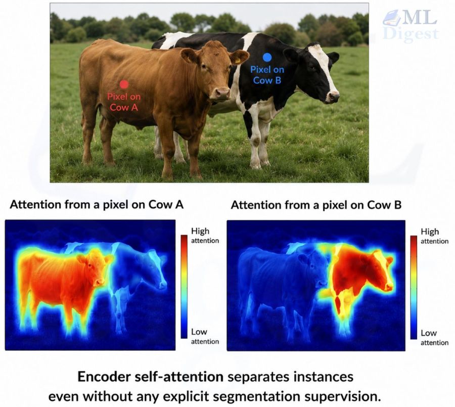
One of the most compelling properties of DETR is the interpretability of its attention maps. Both encoder self-attention and decoder cross-attention tell a coherent story.

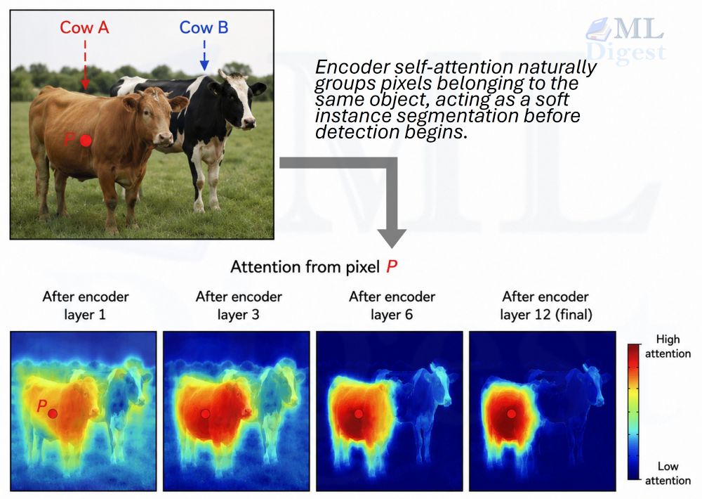
Encoder self-attention. Because the encoder attends globally over the entire image, its attention maps can show instance-aware grouping. If an image has two cows partially occluding each other, the attention map for a pixel on Cow A may highlight much of Cow A while down-weighting Cow B. That is useful qualitative evidence that the encoder is separating context, but it should not be read as DETR explicitly learning an instance-segmentation objective.

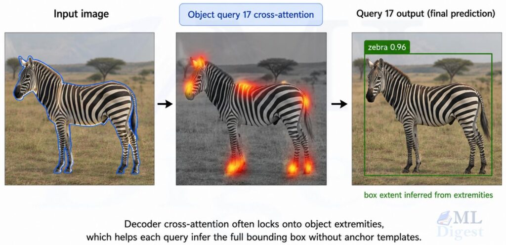
Decoder cross-attention. For each object query that ends up predicting a real object, the cross-attention map shows where in the image that query is “looking.” Queries predicting a zebra strongly attend to the extremities of the zebra (head, hooves, tail) to determine bounding box extent. Background regions receive near-zero attention. This is a qualitatively different behavior from CNN-based detectors, which rely on sliding-window receptive fields.

9. Practical Notes

9.1 Convergence and compute

The original paper highlights that DETR requires significantly longer training schedules than classical detectors. On COCO, competitive DETR results typically require hundreds of epochs, whereas classical detector recipes often converge in a few dozen.

Two factors drive this:

• Global attention over $HW$ tokens is computationally expensive, especially for high-resolution feature maps. This is closely related to the same token-scaling pressure that shows up in Vision Transformers and in practical discussions of how ViT tokens are computed.
• The model must simultaneously learn object representations and the one-to-one assignment behavior. Both take time.

This long optimization horizon was the primary motivation for follow-up work like Deformable DETR.

9.2 What the number of queries $N$ controls

$N$ is a hard upper bound on the number of detectable objects per image. In practice, most scenes have far fewer than $N$ objects, so many queries correctly learn to output the no-object class. Increasing $N$ adds decoder compute linearly but gives the model more capacity for crowded scenes.

9.3 Why the no-object weight matters

Because $N \gg M$ for most images, the path of least resistance for the model is to predict $\varnothing$ everywhere. Down-weighting the no-object class (by $\lambda_{\varnothing} = 0.1$) forces the model to pay proportionally more attention to correctly classifying and localizing the actual objects.

9.4 Where DETR excels

• Scenes with clutter or occlusion, where global context helps disambiguate instances.
• Settings where removing detector-specific engineering (anchors, NMS, proposal stages) is valuable for simplicity or reproducibility.
• Research settings that require a clean, differentiable end-to-end objective.

9.5 Common failure modes of the original DETR

• Weaker performance on small objects compared to large ones. Small objects map to very few tokens in the backbone feature map, and the attention mechanism does not efficiently attend to fine-grained details without multi-scale features.
• Long training schedules.
• High memory pressure as backbone resolution increases, because encoder attention complexity is $O((HW)^2)$.

10. DETR Variants

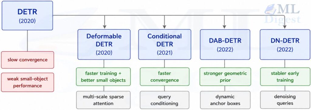
The set-prediction framework proved highly influential. A line of follow-ups addressed the two main weaknesses (slow training, poor small-object detection) while preserving the anchor-free, NMS-free design:

• Deformable DETR (Zhu et al., 2020): Replaces dense attention with sparse, multi-scale deformable attention. It reaches competitive performance in 50 epochs instead of the hundreds of epochs often needed by the original DETR, and it significantly improves small-object AP.
• Conditional DETR (Meng et al., 2021): Modifies query conditioning to provide a clearer geometric signal to the cross-attention, achieving faster convergence.
• DAB-DETR (Liu et al., 2022): Re-parameterizes queries as dynamic anchor boxes, giving the decoder a more explicit geometric prior and improving convergence.
• DN-DETR (Li et al., 2022): Adds query denoising during training to stabilize matching early in training and substantially speed up convergence for DETR-like models.

Summary

DETR is one of the cleaner ideas in modern object detection: treat detection as a set prediction problem, use a Transformer to read the image globally, and use Hungarian matching to enforce one-to-one assignment during training.

The key takeaways are:

• No anchors, no NMS. The set prediction objective makes them unnecessary.
• Object queries are learned, slot-like embeddings that specialize spatially through training.
• Hungarian matching provides the one-to-one supervision signal. It is non-differentiable but that is fine because gradients flow through the loss, not the matching.
• Auxiliary decoder losses are an important training detail, not an optional add-on.
• Trade-off: Elegant architecture, but the original model trains slowly and struggles with small objects. The follow-up literature (Deformable DETR and beyond) addresses both.

S L Happy

Machine Learning Engineer at HP | Website |  + postsBio ⮌

Happy is a seasoned ML professional with over 15 years of experience. His expertise spans various domains, including Computer Vision, Natural Language Processing (NLP), and Time Series analysis. He holds a PhD in Machine Learning from IIT Kharagpur and has furthered his research with postdoctoral experience at INRIA-Sophia Antipolis, France. Happy has a proven track record of delivering impactful ML solutions to clients.

• S L Happy

  BM25 Made Easy: Visualizing the Core of Modern Search
• S L Happy

  What Are Knowledge Graph-Based RAG Systems? Complete Beginner’s Guide
• S L Happy

  EfficientNet Made Easy: Accuracy Through Principled Scaling
• S L Happy

  Evaluation Metrics in Machine Learning: A Practical Field Guide

Silpa

Website |  + postsBio ⮌

Silpa brings 5 years of experience in working on diverse ML projects, specializing in designing end-to-end ML systems tailored for real-time applications. Her background in statistics (Bachelor of Technology) provides a strong foundation for her work in the field. Silpa is also the driving force behind the development of the content you find on this site.

• Silpa

  BM25 Made Easy: Visualizing the Core of Modern Search
• Silpa

  What Are Knowledge Graph-Based RAG Systems? Complete Beginner’s Guide
• Silpa

  EfficientNet Made Easy: Accuracy Through Principled Scaling
• Silpa

  Evaluation Metrics in Machine Learning: A Practical Field Guide