Paper: Rich feature hierarchies for accurate object detection and semantic segmentation (Girshick, Donahue, Darrell, Malik, 2014)
Think of object detection as a game of “Where is it, and what is it?”
- Where: find a bounding box that tightly wraps an object.
- What: assign the correct class label (dog, car, person, etc.).
Before R-CNN, many detectors tried to slide a window over the entire image at many scales and aspect ratios, which is conceptually simple but computationally expensive and often inaccurate. R-CNN introduced a powerful alternative: first propose a few thousand promising regions, then classify each region using a CNN.
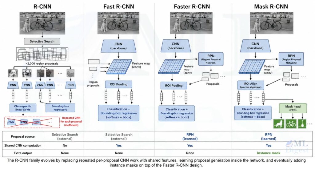
R-CNN (Girshick et al., 2014) was a major stepping stone toward modern detectors (Fast R-CNN, Faster R-CNN, Mask R-CNN). It is not the fastest approach today, but it is historically and conceptually important because it established the “region proposals + deep features” template.
1. What problem does R-CNN solve?
Object detection asks two questions at once:
- Where is the object?
- What is the object?
Given an image, the detector returns a set of predictions of the form:
$$
{(b_i, c_i, s_i)}_{i=1}^{N}
$$
where:
- $b_i$ is a predicted bounding box
- $c_i$ is the predicted class label
- $s_i$ is the confidence score
This is what makes detection harder than plain image classification. A classifier returns one label for the whole image, but a detector may need to return many objects from different categories in different locations.
Why that was hard before R-CNN
Before R-CNN, one common detection strategy was the sliding window approach. A model would scan many locations, scales, and aspect ratios across the image. That idea is conceptually simple, but it is computationally expensive and often wastes effort on background regions.
R-CNN introduced a better division of labor:
- Use Selective Search to generate a few thousand category-agnostic region proposals.
- Warp each proposed region to a fixed size and feed it through a CNN.
- Use the resulting feature vector for classification and bounding-box refinement.
That sounds straightforward today, but in 2014 it was a major shift. Deep networks had already transformed image classification through AlexNet, yet object detection still needed a strong recipe for handling localization. R-CNN was that recipe.
2. The core intuition
I find it useful to think about R-CNN as a three-person team:
- The proposal stage says, “These are the places worth checking.”
- The CNN says, “This crop looks like a car, a dog, or pure background.”
- The regressor says, “The object is here, but the box should move slightly left, upward, and become narrower.”
The important design choice is that R-CNN does not ask the CNN to solve the whole detection problem in one step. It asks the CNN to produce a strong representation for each candidate crop. Once that representation is available, classical machine learning components such as linear Support Vector Machines (SVMs) and linear regressors can finish the job.
The six-step pipeline at a glance
You can summarize R-CNN as a simple funnel:
- Generate candidate regions that might contain an object.
- Normalize each candidate into a fixed-size input for a CNN.
- Extract CNN features for each candidate.
- Classify each candidate (object class vs background).
- Refine the candidate box (bounding-box regression).
- Remove duplicates (non-maximum suppression).
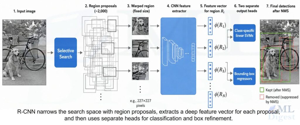
3. The original R-CNN pipeline
3.1 Region proposals
Given an input image $I$, R-CNN first generates a set of region proposals:
$$
\mathcal{R} = {R_1, R_2, \dots, R_N}
$$
where $N$ is typically around 2,000 proposals per image when using Selective Search.
Selective Search is not a neural network. It is a bottom-up grouping algorithm that merges superpixels based on similarity cues such as color, texture, size, and fill. The output is a set of candidate boxes that has high recall, which means the true object is likely to be covered by at least one proposal.
In a bit more detail, it first over-segments the image into many small regions and then repeatedly merges neighboring regions based on cues such as color, texture, size, and fill. The result is a hand-engineered proposal generator with strong recall, but it also adds a noticeable CPU-side runtime cost.
This first stage is critical. If no proposal sufficiently overlaps the object, the later classifier and regressor never get a chance to recover it.
3.2 Warping each proposal and extracting CNN features
Each proposal $R_i$ is cropped from the image and warped to a fixed spatial size. In the original paper, the crop is resized to $227 \times 227$ to match the ImageNet pretrained AlexNet-style input.
This fixed-size warping is convenient for the CNN, but it can distort the aspect ratio of the original object. R-CNN tolerated that distortion surprisingly well, even though later methods tried to preserve geometry more carefully.
The CNN then maps the region to a feature vector:
$$
\phi(R_i) \in \mathbb{R}^d
$$
where $d$ is typically the dimensionality of a high-level fully connected layer, for example 4096 in the original architecture.
Conceptually, $\phi(R_i)$ is the semantic summary of the proposal. If the crop contains a dog head, the feature vector should encode that strongly. If it contains only grass, the vector should look more like background. In the original AlexNet-based setup, these features were often taken from the fc7 layer.
The expensive part is that this CNN pass happens separately for every proposal. With roughly 2,000 proposals, inference means roughly 2,000 forward passes per image.
3.3 Classifying each region
For each object class $c$, R-CNN trains a linear SVM on top of the CNN features. The score for proposal $R_i$ and class $c$ is:
$$
s_{i,c} = w_c^\top \phi(R_i) + b_c
$$
where:
- $w_c$ is the learned weight vector for class $c$
- $b_c$ is the bias term
- $\phi(R_i)$ is the CNN feature vector for proposal $R_i$
The detector assigns a confidence score to each class for each proposal. During inference, proposals with low scores are discarded, and overlapping detections are filtered with non-maximum suppression.
The original R-CNN pipeline also used stricter labels for SVM training than for CNN fine-tuning:
- Positives: ground-truth boxes for that class
- Negatives: proposals with IoU less than 0.3 against every ground-truth instance of that class
- Ignored: intermediate-overlap proposals that are not ground truth
This separation helps the SVM learn a sharper class boundary instead of treating near-miss boxes as fully negative examples.
Because background proposals greatly outnumber object proposals, hard negative mining is important. In practice, the SVM is trained iteratively, and the most confidently misclassified background regions are added back into training as difficult negatives.
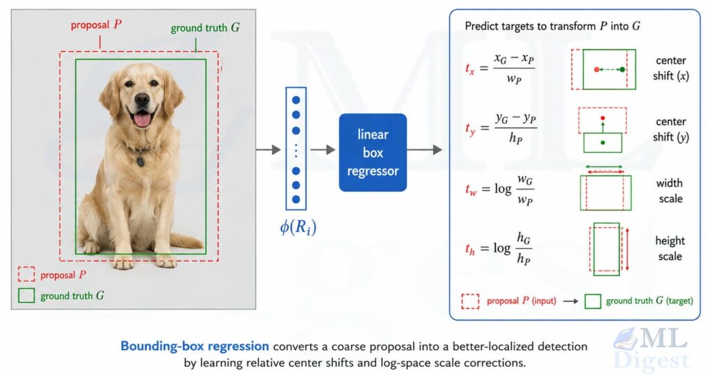
3.4 Refining the bounding boxes
The proposal boxes are rarely perfect, so R-CNN learns a class-specific linear bounding-box regressor.
Suppose a proposal box is:
$$
P = (x_p, y_p, w_p, h_p)
$$
and the matched ground-truth box is:
$$
G = (x_G, y_G, w_G, h_G)
$$
where $(x_G, y_G)$ denotes the center and $(w_G, h_G)$ denotes width and height. The regression targets are encoded as:
$$
t_x = \frac{x_G – x_p}{w_p}, \qquad
t_y = \frac{y_G – y_p}{h_p}, \qquad
t_w = \log\left(\frac{w_G}{w_p}\right), \qquad
t_h = \log\left(\frac{h_G}{h_p}\right)
$$
The regressor predicts $\hat{t} = (\hat{t}_x, \hat{t}_y, \hat{t}_w, \hat{t}_h)$ from the feature vector $\phi(R_i)$. At inference time, the box is decoded back into image coordinates:
$$
\hat{x} = x_p + w_p \hat{t}_x, \qquad
\hat{y} = y_p + h_p \hat{t}_y, \qquad
\hat{w} = w_p \exp(\hat{t}_w), \qquad
\hat{h} = h_p \exp(\hat{t}_h)
$$
This parameterization is still widely used in modern detectors because it makes translation and scale adjustments easier to learn.
The log-space width and height terms are especially useful because scale errors should be learned relatively, not absolutely. A ten-pixel correction means very different things for a tiny box and a large box.
In the original system, these corrections were usually learned with class-specific linear regressors on top of the CNN features.
3.5 Removing duplicates with non-maximum suppression
R-CNN usually produces many overlapping detections around the same object. Non-maximum suppression (NMS) removes those duplicates.
For a single class, the usual loop is:
- Sort detections by score in descending order.
- Keep the highest-scoring box.
- Remove any remaining box whose IoU with that box exceeds a threshold.
- Repeat until no candidates remain.
This post-processing step is simple, but it changes detector behavior quite a lot. A more aggressive threshold removes duplicates more aggressively but can also hurt recall when two true objects are close together.
4. Training R-CNN step by step
One reason R-CNN is historically important is that it was effective despite a fairly awkward training pipeline. It was not end-to-end in the modern sense.
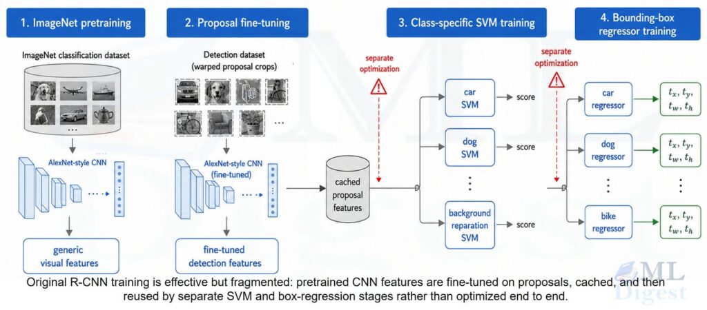
4.1 Step 1: supervised pretraining
The CNN is first pretrained for image classification on ImageNet. This stage teaches the network broadly useful visual features such as edges, textures, parts, and object-level patterns.
That backbone story kept evolving after R-CNN. The jump from AlexNet-depth to much deeper networks became practical once residual connections solved the vanishing-gradient problem at scale. Today, newer feature extractors such as EfficientNet, ConvNeXt, Swin Transformer, Vision Transformer, and self-supervised approaches like DINO can all provide richer visual representations than the original AlexNet-era setup.
Without this pretraining, R-CNN would have struggled because detection datasets at the time were much smaller than classification datasets.
4.2 Step 2: domain-specific fine-tuning on proposals
The pretrained CNN is then fine-tuned on warped region proposals from the detection dataset.
Operationally, the ImageNet classification head is replaced with a new detection head over $N + 1$ classes, meaning $N$ foreground classes plus one background class.
Proposal labels are assigned using Intersection over Union (IoU):
$$
\operatorname{IoU}(A, B) = \frac{|A \cap B|}{|A \cup B|}
$$
In the original recipe, a proposal is treated as a positive example if its IoU with a ground-truth box is at least 0.5, and as background otherwise. This is a looser definition than the later SVM stage, which is one reason the fine-tuning stage can use more positive examples and avoid overfitting the CNN too aggressively.
The fine-tuned CNN learns to produce features that are much more useful for detection than plain ImageNet classification features.
4.3 Step 3: train class-specific SVMs
Once proposal features are extracted and cached, one linear SVM per class is trained on top of those features. Here the label rules become stricter: true positives are the ground-truth boxes for the class, clear background proposals are negatives, and ambiguous in-between overlaps are ignored. Hard negative mining is especially important because most proposals are background.
The SVM objective for class $c$ is typically written as:
$$
\min_{w_c, b_c} \frac{1}{2}|w_c|^2 + C \sum_i \max\left(0, 1 – y_i(w_c^\top \phi(R_i) + b_c)\right)
$$
where $y_i \in {-1, +1}$ is the label for proposal $R_i$.
The $\frac{1}{2}|w_c|^2$ term is an L2 regularization penalty that prevents the SVM weights from growing too large. The hinge loss term $\max(0, 1 – y_i(\cdot))$ is one of several loss designs explored in neural network loss functions.
4.4 Step 4: train bounding-box regressors
Finally, a regression model is fit for each class using positive proposals only. The input is again the CNN feature vector, and the target is the four-parameter box transform. In the original presentation this is commonly described as a linear least-squares style fit on top of frozen CNN features.
This means the original R-CNN has multiple disjoint training stages:
- CNN pretraining
- CNN fine-tuning for detection
- SVM training
- Box regressor training
That complexity is one of the main reasons later models replaced it.
4.5 How R-CNN is evaluated
Detection quality is usually summarized with mean Average Precision (mAP). If you want a broader refresher on how ML metrics behave outside detection, see evaluation metrics in machine learning. On classic PASCAL VOC evaluation, a detection is treated as correct if:
- the predicted class matches the ground-truth class
- the predicted box has IoU at least 0.5 with an unmatched ground-truth box
This is important because R-CNN is not only about classification quality. It must also localize the object well enough to satisfy the IoU criterion.
5. Why R-CNN worked so well
R-CNN succeeded because it combined three ideas that fit together unusually well:
High-recall proposals: The Selective Search algorithm produced a small set of candidate boxes that covered most true objects. That meant the CNN and SVM only needed to focus on a few thousand regions rather than millions of sliding windows.
Strong transferable CNN features: Deep features from ImageNet pretraining generalized far beyond whole-image classification. This was the real breakthrough. A region crop from a detection task could be represented by a feature vector that already knew a lot about visual semantics.
Decoupling representation learning from final decision rules: The CNN produced the representation, while the SVM and regressor handled the final geometry and decision boundaries. That separation was clunky, but it was effective and easy to reason about.
6. The limitations that led to Fast and Faster R-CNN
R-CNN is important, but it is also slow.
- Inference is repetitive: If an image has about 2,000 proposals, the CNN runs about 2,000 times, once per crop. Many of those crops overlap heavily, so the same pixels are processed again and again.
- Training is fragmented: The model is not trained jointly from image to final detection score. Features are extracted, saved to disk, reused for SVMs, and then reused again for regressors.
- Storage costs are large: The original pipeline often cached features for millions of proposals. Historically, this could require hundreds of gigabytes of storage.
- Proposal generation is external: Selective Search is hand-engineered and relatively slow. The detector depends on an external algorithm rather than learning proposals inside the model.
- Compute and memory profile: The bottleneck can be summarized very directly:
- Proposals per image: roughly 2,000
- CNN passes per image: roughly 2,000
- Feature storage: potentially hundreds of gigabytes when caching large proposal sets
This is why the original system was historically important but operationally awkward. The repeated CNN work dominates inference, and the cached-feature workflow dominates training complexity.
7. Major variants of R-CNN
The R-CNN family is easiest to understand as a sequence of fixes to the original pipeline. Each variant keeps the core idea of region-based detection, but removes a different bottleneck.
Fast R-CNN fixed the repeated CNN computation by running the CNN once on the whole image and then pooling features for each region. Faster R-CNN went further by learning proposals with a Region Proposal Network, which made the whole system much faster and more integrated. Mask R-CNN added a parallel segmentation head to predict pixel-level masks for each detected instance.
The progression is easier to remember in plain language:
- R-CNN uses Selective Search, runs the CNN once per proposal, and pays for that modularity with very slow inference.
- Fast R-CNN still uses external proposals, but it shares CNN computation across the whole image and trains the detector much more cleanly.
- Faster R-CNN learns proposals with an RPN, shares the backbone, and turns the detector into a much more unified system.
- Mask R-CNN adds a parallel segmentation head to predict instance masks, while keeping the Faster R-CNN design for detection.
7.1 Fast R-CNN
Fast R-CNN keeps external region proposals, typically from Selective Search, but it stops running the CNN separately on every crop. Instead, the whole image is passed through the backbone once to produce a shared convolutional feature map.
Each proposal is then projected onto that shared feature map, and a Region of Interest pooling layer extracts a fixed-size feature representation for the proposal. Classification and bounding-box regression are trained jointly inside one network, which makes training simpler and inference much faster than original R-CNN.
The key improvement is shared computation. Instead of thousands of CNN forward passes per image, Fast R-CNN does one backbone pass and reuses the resulting features for all proposals.
7.2 Faster R-CNN
Faster R-CNN addresses the next bottleneck: proposal generation. Rather than depending on Selective Search, it learns proposals with a Region Proposal Network (RPN) that runs on top of the same shared convolutional features used by the detector.
This makes the system much more integrated. The backbone computes image features once, the RPN proposes candidate boxes, and the detection head classifies and refines them. Because the proposal stage is now learned and GPU-friendly, Faster R-CNN is both faster and usually more accurate than Fast R-CNN.
Conceptually, Faster R-CNN turns region proposal generation from a hand-engineered preprocessing step into part of the model itself.
7.3 Mask R-CNN
Mask R-CNN extends Faster R-CNN beyond bounding boxes. In addition to class labels and box coordinates, it predicts a pixel-level segmentation mask for each detected instance.
Architecturally, it adds a parallel mask head for each Region of Interest and replaces the coarse ROI Pooling step with ROI Align, which preserves spatial alignment more accurately. That alignment matters because a segmentation mask is much more sensitive to small coordinate errors than a class label is.
The important idea is that Mask R-CNN is not a different detection philosophy. It is a Faster R-CNN style detector with an extra per-instance segmentation branch.
8. A minimal runnable R-CNN-style implementation
The following example is intentionally didactic. It is not a faithful reproduction of the original training pipeline, because that would require a labeled detection dataset, feature caching, SVM training, and box regression. Instead, it demonstrates the central R-CNN idea during inference:
- Generate region proposals.
- Crop each proposal.
- Classify each crop independently with a pretrained CNN.
- Keep high-confidence proposals for one target class.
- Apply non-maximum suppression.
Install the dependencies first:
pip install opencv-contrib-python pillow matplotlib torch torchvisionNow run this script. Set image_path to your local image and choose a category name from the pretrained ImageNet label list bundled with TorchVision.
from pathlib import Path

import cv2
import matplotlib.pyplot as plt
import numpy as np
import requests
import torch
from PIL import Image
from torchvision.models import ResNet50_Weights, resnet50
from torchvision.ops import nms


def selective_search_boxes(image_bgr, max_proposals=300):
    """Generate region proposals with OpenCV selective search."""
    search = cv2.ximgproc.segmentation.createSelectiveSearchSegmentation()
    search.setBaseImage(image_bgr)
    search.switchToSelectiveSearchFast()
    rects = search.process()

    boxes = []
    seen = set()
    for x, y, w, h in rects:
        if w < 32 or h < 32:
            continue
        key = (int(x), int(y), int(w), int(h))
        if key in seen:
            continue
        seen.add(key)
        boxes.append((x, y, x + w, y + h))
        if len(boxes) >= max_proposals:
            break
    return boxes


def draw_boxes(image_rgb, boxes, scores, class_name):
    """Render final detections for inspection."""
    plt.figure(figsize=(10, 8))
    plt.imshow(image_rgb)
    ax = plt.gca()
    for (x1, y1, x2, y2), score in zip(boxes, scores):
        ax.add_patch(
            plt.Rectangle(
                (x1, y1),
                x2 - x1,
                y2 - y1,
                fill=False,
                edgecolor="lime",
                linewidth=2,
            )
        )
        ax.text(x1, y1 - 4, f"{class_name}: {score:.2f}", color="lime", fontsize=10)
    plt.axis("off")
    plt.tight_layout()
    plt.show()


def load_image(url: str) -> Image.Image:
    """Download and convert an image to RGB."""
    response = requests.get(url, stream=True, timeout=30)
    response.raise_for_status()
    return Image.open(response.raw).convert("RGB")


def main():
    image_url = "http://images.cocodataset.org/val2017/000000039769.jpg"
    target_label = "Egyptian cat"
    score_threshold = 0.35
    proposal_limit = 250

    device = "cuda" if torch.cuda.is_available() else "cpu"

    weights = ResNet50_Weights.DEFAULT
    model = resnet50(weights=weights).to(device).eval()
    preprocess = weights.transforms()
    categories = weights.meta["categories"]

    if target_label not in categories:
        raise ValueError(
            f"'{target_label}' is not in the ImageNet label list. "
            "Pick an exact category name from weights.meta['categories']."
        )
    target_index = categories.index(target_label)

    image_pil = load_image(image_url)
    image_rgb = np.array(image_pil) # Convert PIL image to numpy array for matplotlib
    image_bgr = cv2.cvtColor(image_rgb, cv2.COLOR_RGB2BGR) # Convert to BGR for OpenCV functions like selective search

    proposals = selective_search_boxes(image_bgr, max_proposals=proposal_limit)

    kept_boxes = []
    kept_scores = []

    with torch.inference_mode():
        for x1, y1, x2, y2 in proposals:
            crop = image_rgb[y1:y2, x1:x2]
            if crop.size == 0:
                continue

            crop_pil = Image.fromarray(crop)
            tensor = preprocess(crop_pil).unsqueeze(0).to(device)
            logits = model(tensor)
            probs = torch.softmax(logits, dim=1)[0]
            score = probs[target_index].item()

            if score >= score_threshold:
                kept_boxes.append([x1, y1, x2, y2])
                kept_scores.append(score)

    if not kept_boxes:
        print("No detections survived the score threshold.")
        return

    boxes_tensor = torch.tensor(kept_boxes, dtype=torch.float32)
    scores_tensor = torch.tensor(kept_scores, dtype=torch.float32)
    keep = nms(boxes_tensor, scores_tensor, iou_threshold=0.3)

    final_boxes = boxes_tensor[keep].int().tolist()
    final_scores = scores_tensor[keep].tolist()
    draw_boxes(image_rgb, final_boxes, final_scores, target_label)


if __name__ == "__main__":
    main()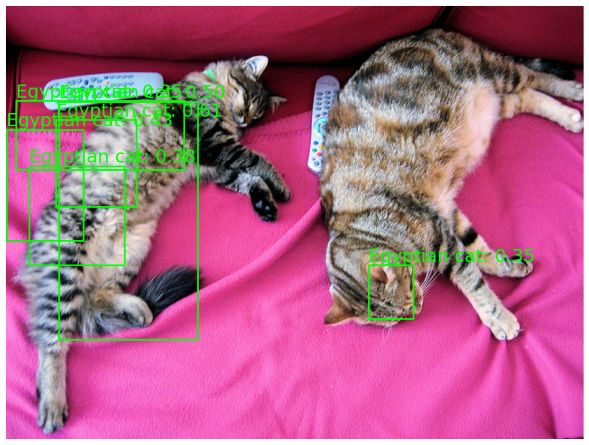
What this script teaches correctly:
- Detection can be decomposed into proposal generation, crop-wise feature extraction, scoring, and non-maximum suppression.
- Region-based inference is straightforward to reason about and debug.
- Proposal quality matters a great deal, because a missed proposal cannot be recovered later.
What this script simplifies:
- It uses a pretrained classifier directly rather than training detection-specific SVMs.
- It does not learn bounding-box regression.
- It relies on ImageNet class names, which are not the same as a custom detection label space.
- It is much slower than modern detectors because every crop triggers a separate CNN forward pass.
Practical tips and best practices
If you are studying or reproducing R-CNN today, the following habits matter more than fancy implementation details:
- Start with a small subset of data and verify proposal quality visually before training anything.
- Cache proposal coordinates and proposal-to-ground-truth matches, because recomputing them repeatedly is wasteful.
- Use a balanced sampling strategy during fine-tuning, because raw proposals are overwhelmingly background.
- Inspect false positives after non-maximum suppression. Many apparent classifier problems are really proposal problems.
- Keep the region preprocessing consistent with the pretrained backbone. With TorchVision models, prefer the official
weights.transforms()pipeline over hand-written normalization. - If your goal is production object detection rather than historical understanding, use Faster R-CNN, RetinaNet, YOLO, or DETR-style models instead.
Summary
R-CNN was a turning point in computer vision because it showed how to combine high-recall region proposals with deep convolutional features for accurate object detection. Its pipeline was not elegant, but it was decisive: propose regions, encode each region with a CNN, score those features class by class, and refine the box geometry.
The details that made it work are worth remembering: Selective Search supplied high-recall proposals, the CNN provided transferable deep features, the SVM stage used strict labels with hard negative mining, the box regressor corrected coarse localization, and NMS turned many overlapping hypotheses into a usable final prediction set.

Silpa brings 5 years of experience in working on diverse ML projects, specializing in designing end-to-end ML systems tailored for real-time applications. Her background in statistics (Bachelor of Technology) provides a strong foundation for her work in the field. Silpa is also the driving force behind the development of the content you find on this site.
Subscribe to our newsletter!