Swin Transformer Made Easy: A Hierarchical Vision Transformer with Shifted Windows

Paper: Swin Transformer: Hierarchical Vision Transformer using Shifted Windows (Liu et al., 2021), Swin Transformer V2: Scaling Up Capacity and Resolution (Liu et al., 2022)
Reference Implementations: Microsoft Swin Transformer repository , timm, torchvision vision transformer docs

Imagine reading a large city map through a small square window cut into a sheet of paper. You can inspect one neighborhood at a time very efficiently, but you miss how nearby neighborhoods connect. Now imagine that after each glance, you slide the window slightly so that the next view overlaps with the previous one. Suddenly, information can flow across neighborhoods without ever needing to view the entire city at once.

I like this mental picture because it captures what Swin Transformer is trying to do without forcing you to stare at an attention matrix on the first paragraph. If you have ever worked with vanilla ViT and felt the cost of global self-attention at high resolution, you are already thinking in the right direction.

That is the core idea behind the Swin Transformer paper. Instead of applying global self-attention across all image patches, which becomes expensive at high resolution, Swin Transformer computes attention inside small local windows and then shifts those windows between blocks. This simple change makes transformers practical as general-purpose vision backbones for classification, object detection, and segmentation.

I will walk you through why Swin Transformer matters, how the shifted-window mechanism works, the math behind its efficiency, and how Swin Transformer V2 extends the design. By the end, you will understand not only what the architecture does, but also why so many practitioners consider it the first transformer backbone suitable for a production vision stack.

1. Why Swin Transformer Matters

Before Swin Transformer, Vision Transformer (ViT) showed that pure transformers could perform extremely well on image classification. However, the original ViT had two practical limitations:

1. It used global self-attention, whose cost grows quadratically with the number of image tokens.
2. It kept a single-scale representation, which is less natural for dense vision tasks such as detection and segmentation.

These two issues matter a lot in computer vision. High-resolution images generate many tokens, and tasks like detection need a feature pyramid with multiple spatial scales.

If you want a quick feel for how fast that token count grows as image resolution changes, it helps to work through a few examples from computing Vision Transformer tokens.

Swin Transformer addresses both issues directly:

1. Window-based attention reduces the attention cost by restricting attention to local regions.
2. Shifted windows allow information exchange across neighboring windows.
3. Hierarchical stages with patch merging create multi-scale feature maps, much like a CNN backbone.

This is why Swin Transformer quickly became an important backbone in systems built on top of Mask R-CNN, UPerNet, and related dense prediction pipelines. In my experience, this is the point where Swin stops feeling like “another transformer paper” and starts feeling like a serious systems paper for vision.

If you want a transformer-native comparison point on the detection side, DETR is a useful contrast because it pushes transformer ideas directly into object detection rather than using Swin primarily as a backbone.

The follow-up Swin Transformer V2 kept the same high-level recipe, local windows, shifted communication, and hierarchical stages, but made it much easier to scale that recipe to larger models and higher-resolution inputs. That matters because the original Swin idea solves the efficiency problem, while V2 spends more of its effort on the equally practical question of how to keep optimization stable when your ambition grows.

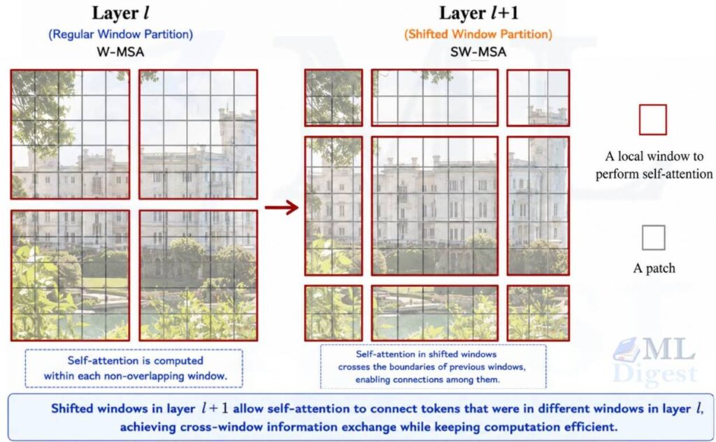
2. Intuition First: Local Meetings, Then Neighborhood Coordination

Think of an image as a large company. Each image patch is one employee. Global self-attention is like asking every employee to attend the same all-hands meeting every time a decision is needed. That is flexible, but expensive and noisy.

Swin Transformer replaces that with local meetings:

1. In one block, employees only talk to others in their immediate team, which is a fixed window.
2. In the next block, the team boundaries shift slightly.
3. Because of that shift, employees who were in different teams before can now interact.

After a few alternating blocks, information spreads across the image without paying the full cost of global attention. You still get communication beyond one local region, just without forcing every patch to gossip with every other patch immediately.

This is the main engineering insight of Swin Transformer. It keeps the transformer machinery, but organizes communication in a way that better matches image structure. I think that is one reason the paper aged well, it did not win by being flashy, it won by being disciplined.

3. The Big Architectural Idea

Swin Transformer combines three ideas into one backbone:

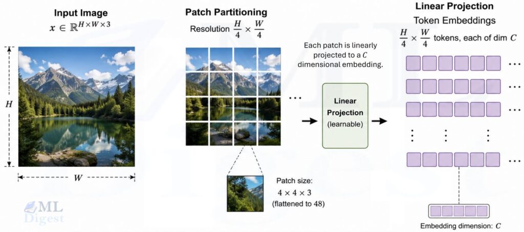
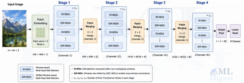
3.1 Patch Embedding

Like ViT, Swin begins by splitting an image into non-overlapping patches. The common setup uses a patch size of 4. If you are coming from CNNs, you can think of this as a very assertive first convolution that immediately says, “We are operating on tokens now.”

For an input image $x \in \mathbb{R}^{H \times W \times 3}$, patch partitioning produces tokens at resolution $\frac{H}{4} \times \frac{W}{4}$. Each patch is linearly projected into an embedding vector of size $C$.

In practice, this is usually implemented with a convolution:

$$
\operatorname{PatchEmbed}(x) = \operatorname{Conv2D}(3, C, \operatorname{kernel}=4, \operatorname{stride}=4)(x)
$$

This is efficient and directly maps image patches into token embeddings.

3.2 Hierarchical Stages

Unlike the original ViT, Swin does not keep one fixed token resolution throughout the network. Instead, it builds a hierarchy of stages:

1. Stage 1 operates at resolution $H/4 \times W/4$.
2. Stage 2 operates at resolution $H/8 \times W/8$.
3. Stage 3 operates at resolution $H/16 \times W/16$.
4. Stage 4 operates at resolution $H/32 \times W/32$.

Between stages, a patch merging layer reduces spatial resolution (number of tokens) and increases the channel dimension. Patch Merging layer acts like a pooling layer in a CNN. It:

• Reduces spatial resolution by half (H/4→H/8 and W/4→W/8).
• Increases channel depth by double (C→2C).

This is carried out by taking 2 x 2 groups of neighboring tokens, concatenating their features, and applying a linear projection. The result is a new set of tokens that represent larger receptive fields with richer semantics.

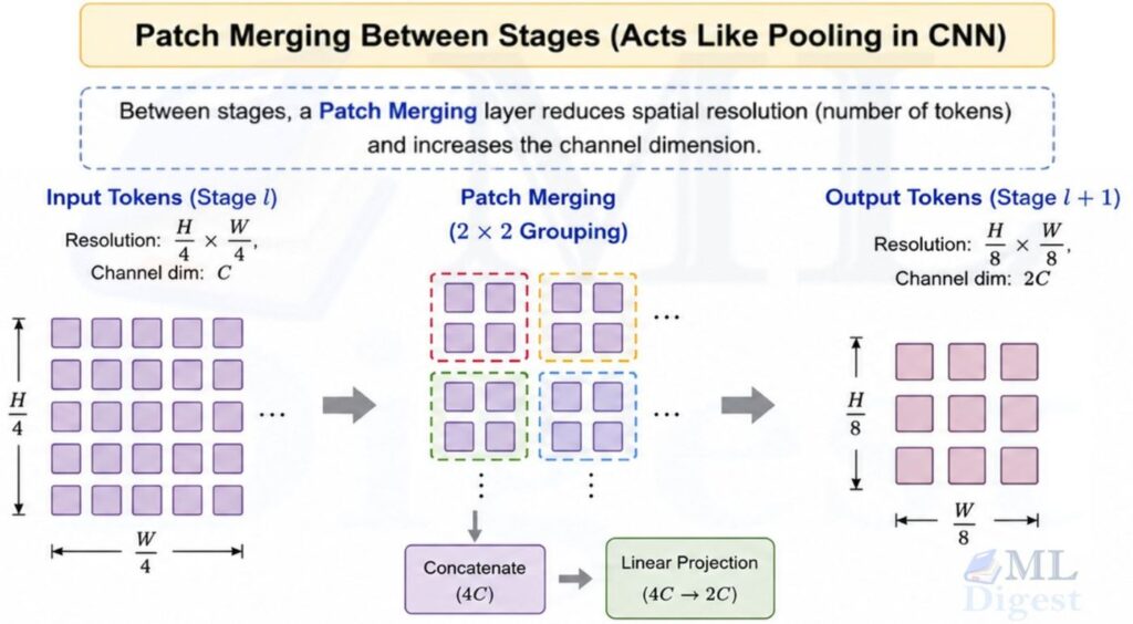
a) Grid Partitioning (Grouping)

Imagine a grid of feature tokens of size $H/4 \times W/4$ with $C$ channels. The layer divides this grid into $2 \times 2$ local neighborhoods. Within every $2 \times 2$ block, it selects pixels based on their relative positions.

b) Concatenation

Next, these 4 downsampled token maps are concatenated along the channel dimension.

$$\text{Concatenated Size:} \quad \left(\frac{H}{8} \times \frac{W}{8}\right) \times 4C$$

Unlike max or average pooling, Patch Merging first concatenates the four neighboring token vectors so the next projection can learn how to compress that local information. It does not preserve all information losslessly, because the concatenated $4C$ channels are then projected down to $2C$.

c) Linear Projection (Reduction)

Having $4C$ channels can quickly become computationally expensive for the upcoming self-attention layers. To fix this, Swin Transformer applies a Linear Layer (a matrix multiplication) to project the $4C$ channels down to $2C$ channels.

To put it mathematically, the tensor transforms like this through a Patch Merging layer (in stages 1 to 2, for example):

$$\text{Input: } (H/4, W/4, C) \xrightarrow{\text{Group \& Concatenate}} \left(\frac{H}{8}, \frac{W}{8}, 4C\right) \xrightarrow{\text{Linear Projection}} \left(\frac{H}{8}, \frac{W}{8}, 2C\right)$$

This makes Swin behave much more like a CNN backbone and makes it easy to plug into downstream vision systems.

3.3 Alternating Attention Blocks

Within each stage, Swin alternates between two block types:

1. W-MSA: window-based multi-head self-attention.
2. SW-MSA: shifted-window multi-head self-attention.

This alternating pattern is what enables local efficiency and cross-window communication at the same time. You can think of the first block as “work within the room” and the second block as “now move the walls a little and repeat.”

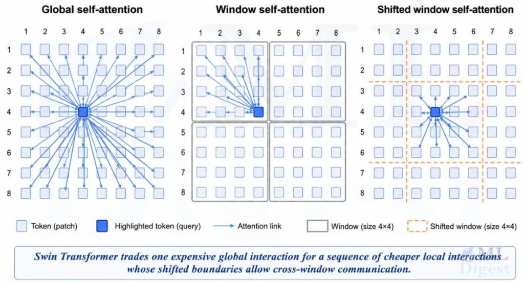
4. Window Attention, Step by Step

4.1 Standard Self-Attention Refresher

Given a token matrix $X \in \mathbb{R}^{N \times C}$, multi-head self-attention first computes queries, keys, and values:

$$
Q = XW_Q, \quad K = XW_K, \quad V = XW_V
$$

For one head, the attention output is:

$$
\operatorname{Attention}(Q, K, V) = \operatorname{Softmax}\left(\frac{QK^T}{\sqrt{d}}\right)V
$$

where $d$ is the head dimension. This is the standard scaled dot-product attention formulation.

The problem is that the attention matrix $QK^T$ has shape $N \times N$. If $N$ is large, the computation and memory cost grow quadratically with the number of tokens.

4.2 Window-Based Multi-Head Self-Attention (W-MSA)

Swin partitions the feature map into non-overlapping windows of size $M \times M$. Attention is computed independently inside each window.

If the feature map has $h \times w$ tokens, then the complexity of global attention is:

$$
\Omega(\text{MSA}) = 4hwC^2 + 2(hw)^2C
$$

For window attention, the complexity becomes:

$$
\Omega(\text{W-MSA}) = 4hwC^2 + 2M^2hwC
$$

This is the crucial savings. The quadratic term now depends on the fixed window size $M^2$, not on the total number of tokens $hw$. That one change is the reason you can seriously consider Swin for larger images instead of treating it as a beautiful but impractical idea.

If $M = 7$, which is common in the original paper, the cost remains manageable even for large images.

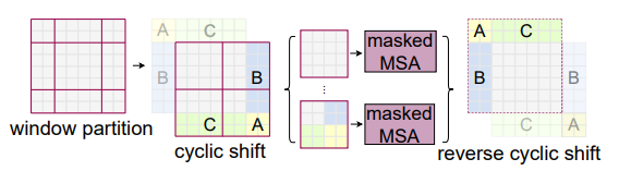
4.3 Shifted Window Multi-Head Self-Attention (SW-MSA)

Pure window attention has one obvious weakness: tokens in different windows do not interact.

Swin fixes that by shifting the window partition in the next block. In the original design, the shift size is usually half the window size, so with $M = 7$, the shift is often 3.

Operationally, the model does this:

1. Cyclically shift the feature map.
2. Partition the shifted map into windows.
3. Compute attention inside each shifted window.
4. Apply an attention mask so that tokens only interact with valid members of the shifted region.
5. Shift the feature map back.

This trick is elegant because it preserves efficient batch computation while allowing cross-window connections. Rather than padding boundaries or processing partial windows separately, a cyclic shift with masking allows the entire feature map to be processed as a uniform batch. The mask prevents attention between tokens that were originally far apart and only became adjacent due to the cyclic wrap.

4.4 Relative Position Bias

Images have strong local spatial structure, so Swin adds a learnable relative position bias to attention logits.

The attention equation becomes:

$$
\operatorname{Attention}(Q, K, V) = \operatorname{Softmax}\left(\frac{QK^T}{\sqrt{d}} + B\right)V
$$

where $B$ is a bias matrix indexed by relative offsets between token pairs inside a window. Since $M^2$ represents the number of patches in a window and relative positions along each axis range from $-M+1$ to $M-1$, the model learns one bias value per relative offset and per attention head. In practice, implementations store this as a compact table with $(2M-1)^2$ relative offsets and $n_H$ heads, then expand it into the full $M^2 \times M^2$ bias matrix used inside attention.

This gives the model a lightweight notion of spatial geometry without using full absolute position embeddings in every stage. In vision, that kind of bias matters because pixels are not a bag of unrelated tokens pretending to be neighbors.

In the original Swin formulation, this bias is stored as a learned table for the fixed relative offsets inside one window. That works well when the training and inference setup stay close to each other. However, when you want to fine-tune at a very different resolution or use a different window size, the bias table becomes one of the places where scaling starts to feel less graceful.

4.5 What Swin Transformer V2 Changes

The original Swin idea was already efficient, but scaling it up exposed three pain points: large attention logits, unstable deep activations, and position-bias parameters that did not transfer cleanly across window sizes.

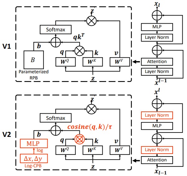
Swin Transformer V2 addresses those issues with three main changes:

1. Residual-post-norm moves normalization to the end of each residual branch, instead of normalizing the branch input first as in the original pre-norm block. In Swin V2, the attention or MLP branch is computed first, normalized, and then added back to the shortcut, which improves stability when scaling depth and model size.
2. Scaled cosine attention is applied instead of scaled dot-product attention. It computes attention scores as the cosine similarity between queries and keys, which keeps them in a more stable range. Plus, a relative position bias is added to the cosine similarity, which gives the model a more direct way to learn spatial relationships without relying on the magnitude of the dot product.
   $$ \text{Sim}(q_i, k_j) = \text{cos}(q_i, k_j) / \tau + B_{ij} $$
   where $\tau$ denotes a learnable scaling term that is typically parameterized per head within each attention module, and $B_{ij}$ is the relative position bias for the token pair $(i, j)$.
3. Log-spaced continuous position bias replaces the discrete lookup table with a smoother function of relative position.

The practical benefit is straightforward. Swin V2 preserves the same local-window backbone that made Swin attractive in the first place, but it is more comfortable when you push model size, window size, or image resolution much harder. If Swin felt like the version that made hierarchical vision transformers deployable, V2 felt like the version that made them scale without getting temperamental.

5. Anatomy of a Swin Transformer Block

Each Swin block follows a pre-normalization transformer pattern built around Layer Normalization:

$$
\hat{z}^{l} = \text{W-MSA}(\text{LN}(z^{l-1})) + z^{l-1}
$$

$$
z^{l} = \text{MLP}(\text{LN}(\hat{z}^{l})) + \hat{z}^{l}
$$

For the shifted version, the attention term changes to SW-MSA:

$$
\hat{z}^{l+1} = \text{SW-MSA}(\text{LN}(z^{l})) + z^{l}
$$

$$
z^{l+1} = \text{MLP}(\text{LN}(\hat{z}^{l+1})) + \hat{z}^{l+1}
$$

The MLP is the standard transformer feed-forward network:

$$
\operatorname{MLP}(x) = W_2\,\sigma(W_1x)
$$

where $\sigma$ is usually GELU.

A Swin block therefore has four key parts:

1. LayerNorm
2. Window attention or shifted-window attention
3. Residual connection
4. MLP with another residual connection

This is still a transformer block. The novelty is how attention is structured spatially.

6. A Concrete Architecture Walkthrough

Swin Transformer scales across four variants corresponding to capacity—Swin-T (Tiny), Swin-S (Small), Swin-B (Base), and Swin-L (Large)—by increasing the base embedding channels $C$ and repeating blocks. They are mathematically differentiated by their base channel dimension $C$ in the first layer and the number of Swin blocks (depths) per stage:

Variant	Embed Dim ($C$)	Depths per Stage	Heads per Stage	Window Size	Params	Target Profile & Applications
Swin-T (Tiny)	96	(2, 2, 6, 2)	(3, 6, 12, 24)	7	~28M	Designed for fast inference and lightweight applications, providing a high-speed backbone for real-time video and edge-scale tasks.
Swin-S (Small)	96	(2, 2, 18, 2)	(3, 6, 12, 24)	7	~50M	Balances accuracy and latency by opening up depth in the third stage, offering richer features without heavy computational costs.
Swin-B (Base)	128	(2, 2, 18, 2)	(4, 8, 16, 32)	7	~88M	The versatile default matching standard ViT-B in size, achieving strong classification performance (~84.5% top-1 ImageNet accuracy).
Swin-L (Large)	192	(2, 2, 18, 2)	(6, 12, 24, 48)	7	~197M	A heavyweight model doubling Swin-T’s channel width, utilized for SOTA accuracy in dense prediction tasks like COCO detection and segmentation (reaching over 87% with ImageNet-22K pretraining).

For an input image of size 224 x 224:

1. Patch embedding produces 56 x 56 tokens with 96 channels.
2. Stage 1 processes those tokens with alternating W-MSA and SW-MSA blocks.
3. Patch merging reduces to 28 x 28 tokens and increases channels to 192.
4. The same pattern repeats until Stage 4 ends at 7 x 7 resolution.
5. Global pooling and a linear head produce the final class logits.

This structure explains why Swin is easy to adapt as a backbone. Each stage emits a feature map at a useful resolution.

If you look at current model zoos, you will often find both Swin and Swin V2 checkpoints. That is not redundancy for its own sake. Original Swin is still the clearest introduction to shifted-window transformers, while V2 is often the safer choice once training scale or fine-tuning resolution starts stretching the original assumptions.

7. Practical Tips and Best Practices

Choose Window Size Deliberately: Window size controls the tradeoff between local context and compute. Larger windows capture more context, but they also increase the per-window attention cost. The standard choice of 7 works well for many image tasks because it provides a good balance.

Cache Attention Masks: For shifted-window attention, mask construction can become an unnecessary overhead if it is rebuilt every iteration. In production code, cache the masks per resolution and reuse them.

Be Careful with Tensor Layout: Educational code often uses channels-last layout $(B, H, W, C)$ because it makes window partitioning and LayerNorm cleaner. Many training pipelines default to channels-first $(B, C, H, W)$. If you mix them, keep the permutations explicit and minimize layout conversions.

Use a Pretrained Backbone for Dense Tasks: If your goal is detection or segmentation, it is usually better to start from an ImageNet-pretrained Swin checkpoint rather than training from scratch. Libraries such as MMDetection and MMSegmentation already provide strong recipes.

Prefer Swin V2 When Resolution or Model Size Jumps: If you expect to fine-tune at much higher resolution than pretraining, or if you plan to use a much larger backbone, Swin V2 is usually the more forgiving starting point. Its continuous position bias transfers more naturally across window configurations, and scaled cosine attention tends to behave better in aggressive scaling regimes.

Understand What Swin Gives You, and What It Does Not: Swin is not global attention in the original ViT sense. It approximates wider communication through repeated local interactions and hierarchical downsampling. That is often exactly what vision needs, but it is still a different inductive bias from fully global attention. If you keep that distinction clear in your head, you will make better decisions about when to use it.

8. Where Swin Transformer Works Well

Swin Transformer is especially strong when you need:

1. A transformer-based backbone that scales to high-resolution images.
2. Multi-scale features for dense prediction.
3. Strong transfer learning across classification, detection, and segmentation.
4. A mature ecosystem with official code and downstream framework support.

It has been widely used in image classification, object detection, semantic segmentation, instance segmentation, video understanding extensions, and medical imaging adaptations.

9. Limits and Tradeoffs

Swin Transformer is powerful, but it is not free of tradeoffs.

1. Window partitioning and shifting add implementation complexity compared with a plain CNN.
2. Local attention is efficient, but it is still more operationally involved than a simple convolution.
3. Performance depends on careful engineering in the attention kernels and mask handling.
4. As you scale the original design to much larger models or much higher image resolutions, optimization and position-bias transfer become harder.

Swin Transformer V2 directly addresses point 4 with scaled cosine attention, residual-post-norm, and log-spaced continuous position bias (see Section 4.5 for details).

The practical takeaway is not that Swin V2 invalidates Swin, or that either model replaces every backbone. Swin made hierarchical transformers viable enough to become first-class backbones in real vision systems, and V2 made that same recipe easier to scale into regimes closer to industrial training pipelines. Both contributions changed what practitioners consider deployable.

Summary

Swin Transformer succeeded because it solved the right engineering problem. It kept the expressive transformer block, but replaced global communication with local window attention and periodic shifted windows. That one design choice dramatically reduced cost while preserving information flow. Combined with patch merging, it also introduced the multi-scale hierarchy that dense vision tasks depend on.

Swin Transformer V2 did not change that backbone philosophy. It made the philosophy scale better. Scaled cosine attention, residual-post-norm, and continuous position bias gave practitioners a cleaner path to larger models and higher-resolution fine-tuning without abandoning the shifted-window design.

If you want to go deeper, the best next step is to read the original Swin Transformer paper, then the Swin Transformer V2 paper, inspect the official implementation, and compare both with ViT and ConvNeXt. If you do that comparison carefully, you will start seeing the real design tradeoffs instead of just memorizing model names.