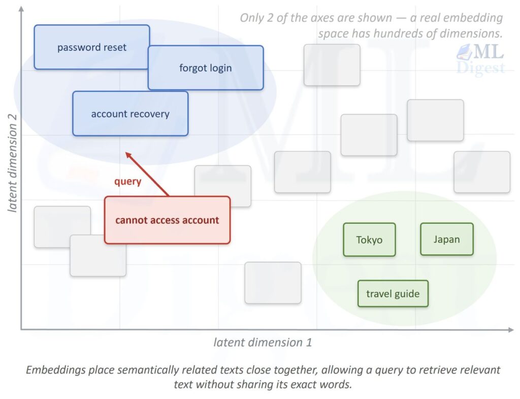
Search breaks down when wording changes but meaning stays the same. A user types “I forgot my credentials,” while the most useful help article is titled “Reset your password“. Keyword overlap is weak, yet the intent is almost identical. A text embedding addresses this problem by mapping each piece of text to a point in a high-dimensional semantic space, where related meanings lie close together even if the words differ.
That geometric view of language is a core building block of modern natural-language systems. Text embeddings let software compare meaning with standard numerical operations, which makes semantic search, recommendations, clustering, classification, duplicate detection, and the retrieval stage of retrieval-augmented generation (RAG) practical at scale. This article explains what text embeddings are, how similarity is measured, how models learn useful vector spaces, and where different embedding approaches fit in practice.
1. What Is a Text Embedding?
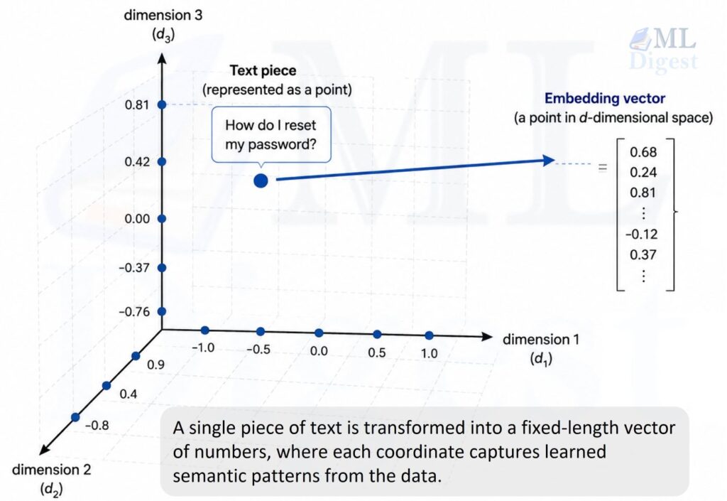
An embedding is a dense vector of real numbers that represents a token, sentence, paragraph, or document:
$$
f(x) = \mathbf{e}_x \in \mathbb{R}^{d}
$$
Here, $x$ is text, $f$ is an embedding model, and $d$ is the embedding dimension. For example, an embedding model could turn a sentence into a vector with 384 or 1,536 coordinates. The coordinates do not have individual human-readable meanings. Instead, their geometry carries information: direction and distance encode patterns learned from text.
Consider these sentences:
- “How do I reset my password?”
- “I cannot log in because I forgot my credentials.”
- “What is the capital of Japan?”
The first two should be nearby on the semantic map. The third should be far away. That is why embeddings improve on exact-keyword matching. A search for “forgot my credentials” can retrieve a help article titled “Reset your password” even though the wording differs.
1.1 Embeddings are not one-hot vectors
A one-hot vector represents a vocabulary item with a long vector containing one $1$ and otherwise $0$s. If a vocabulary has $V$ words, every vector has $V$ dimensions. “cat” and “dog” are equally distant from each other as “cat” and “telescope.” This representation records identity, not similarity.
Dense embeddings use far fewer dimensions and learn their values from data. Related terms tend to receive similar representations. An embedding is also different from a model’s output probability distribution. It is an intermediate numerical representation designed to preserve useful relationships for a task.
2. Why Embeddings Are Useful
Most language is ambiguous and variable. “Cheap flights to Paris,” “low-cost airfare for France,” and “find budget plane tickets” express a similar intent. Rules and keyword lists struggle to cover this variation, and manually maintaining them becomes brittle.
Embeddings provide three practical benefits:
- Semantic matching: compare meanings rather than only overlapping tokens. This is central to semantic retrieval and question answering.
- A reusable feature layer: pass fixed-length numerical features to downstream classifiers, rankers, or clustering algorithms. For example, k-nearest neighbors can route a new support ticket to the right queue by comparing it with similar historical tickets.
- Scalable indexing: precompute document vectors once, store them in a vector index, then search by vector similarity at query time. Approximate nearest-neighbor search makes this feasible for large corpora.
Embeddings are especially valuable when labels are scarce. A team can often start with retrieval or similarity-based grouping before it has enough annotated examples to train a dedicated supervised model.
3. The Geometry Behind Similarity
Once text becomes vectors, similarity is a mathematical choice. The most common metric is cosine similarity:
$$
\operatorname{cosine}(\mathbf{u}, \mathbf{v}) =
\frac{\mathbf{u}^{\mathsf{T}}\mathbf{v}}
{\lVert\mathbf{u}\rVert_2\lVert\mathbf{v}\rVert_2}
$$
Cosine similarity measures the angle between vectors. It is $1$ when they point in the same direction, $0$ when they are orthogonal, and $-1$ when they point in opposite directions. It intentionally discounts vector magnitude, which can be helpful when length should not determine relevance.
Many embedding pipelines normalize vectors to unit length:
$$
\hat{\mathbf{e}} = \frac{\mathbf{e}}{\lVert\mathbf{e}\rVert_2}
$$
For normalized vectors, cosine similarity equals the dot product. It also connects directly to Euclidean distance:
$$
\lVert\hat{\mathbf{u}} – \hat{\mathbf{v}}\rVert_2^2 = 2 – 2\hat{\mathbf{u}}^{\mathsf{T}}\hat{\mathbf{v}}
$$
Detailed Derivation
Derivation: Expand the squared norm using the dot-product definition. For normalized vectors $\hat{\mathbf{u}}$ and $\hat{\mathbf{v}}$ with $\lVert\hat{\mathbf{u}}\rVert_2 = \lVert\hat{\mathbf{v}}\rVert_2 = 1$:
$$
\lVert\hat{\mathbf{u}} – \hat{\mathbf{v}}\rVert_2^2 = (\hat{\mathbf{u}} – \hat{\mathbf{v}})^{\mathsf{T}}(\hat{\mathbf{u}} – \hat{\mathbf{v}})
$$
Expand the product:
$$
= \hat{\mathbf{u}}^{\mathsf{T}}\hat{\mathbf{u}} – 2\hat{\mathbf{u}}^{\mathsf{T}}\hat{\mathbf{v}} + \hat{\mathbf{v}}^{\mathsf{T}}\hat{\mathbf{v}}
$$
Since each vector has unit length:
$$
= 1 – 2\hat{\mathbf{u}}^{\mathsf{T}}\hat{\mathbf{v}} + 1 = 2 – 2\hat{\mathbf{u}}^{\mathsf{T}}\hat{\mathbf{v}}
$$
This means a vector database can use either metric consistently if vectors are normalized and its index is configured correctly. Do not mix a model’s recommended normalization and metric without testing, because retrieval quality can change substantially.
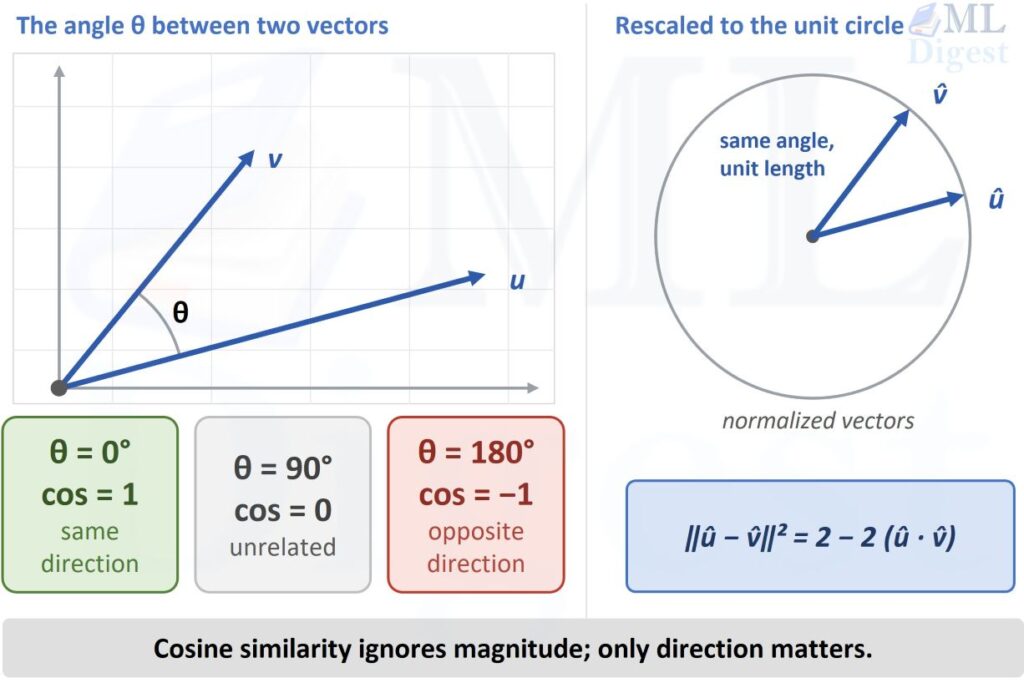
Cosine similarity measures the angle between two embeddings, so normalizing vectors to unit length ties cosine similarity directly to the dot product and to Euclidean distance.
3.1 How models learn a useful space
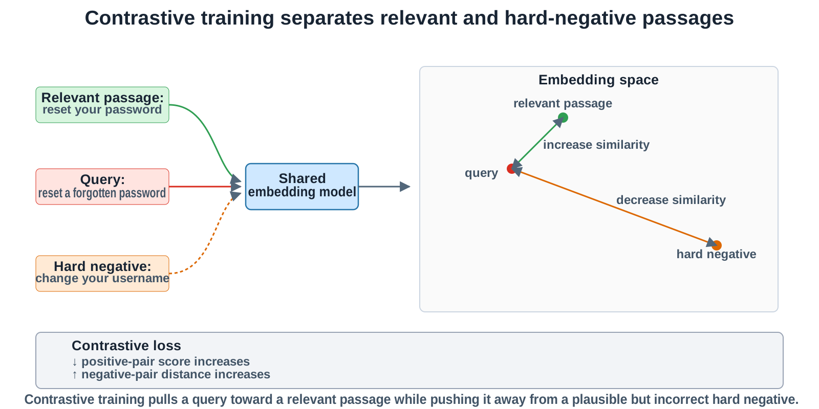
Cosine similarity and distance only tell us how to measure closeness once vectors exist; they say nothing about how a model learns to place related texts near each other in the first place. Embedding training supplies that missing signal: it tells the model which texts should be close and which should not. A common contrastive objective scores a query $q$, a relevant passage $p^+$, and negative passages $p^-_j$:
$$
\mathcal{L} = -\log
\frac{\exp(s(q,p^+)/\tau)}
{\exp(s(q,p^+)/\tau) + \sum_j \exp(s(q,p^-_j)/\tau)}
$$
The score $s$ is often a dot product or cosine similarity, and the temperature parameter $\tau$ controls how sharply the model separates candidates. Minimizing this loss increases the positive pair’s score relative to negatives. Good, difficult negatives, such as a passage about changing a username when the query asks about resetting a password, are particularly informative.
4. Ways to Compute Text Embeddings
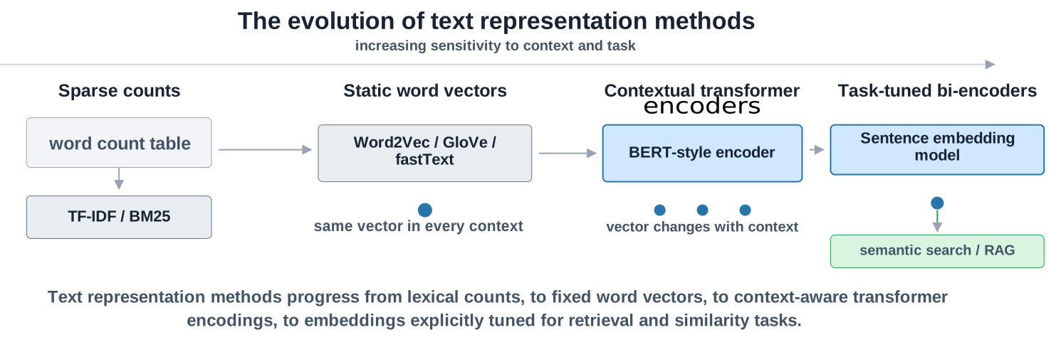
The right approach depends on what “similar” means in the application, the available data, latency limits, languages, and budget. The methods below progress from surface-level word statistics to contextual neural representations.
4.1 Sparse count, TF-IDF, and BM25 representations
The simplest representation counts words or $n$-grams. TF-IDF reduces the importance of common terms and increases the importance of terms distinctive to a document:
$$
\operatorname{tfidf}(t,d) = \operatorname{tf}(t,d)\log\frac{N}{\operatorname{df}(t)}
$$
These vectors are usually high-dimensional and sparse. They work well for exact terms, identifiers, names, error codes, and transparent baseline systems. BM25 extends this family with document-length normalization and remains an exceptionally strong lexical-retrieval baseline.
However, lexical methods do not automatically know that “automobile” relates to “car.” They also cannot make a word’s representation depend on its context.
4.2 Static word embeddings
Methods such as Word2Vec, GloVe, and fastText learn one dense vector per word. Word2Vec’s skip-gram objective predicts nearby context words from a center word. The distributional hypothesis motivates it: words occurring in similar contexts tend to have related meanings.
To embed a sentence, one basic technique averages its word vectors:
$$
\mathbf{e}_{\mathrm{sentence}} = \frac{1}{n}\sum_{i=1}^{n}\mathbf{w}_i
$$
This is cheap and can be a useful baseline, but it loses word order and treats a word identically in every context. “bank” in a financial sentence and “bank” beside a river get the same static vector.
4.3 Contextual transformer embeddings
Contextual models address this limitation directly: instead of one fixed vector per word, they compute a different representation for each occurrence based on its surrounding text. Before a transformer can do this, raw text must first be split into tokens. Most modern encoders rely on a subword algorithm such as byte-pair encoding, which keeps common words intact while breaking rare words into smaller reusable pieces so the model can still represent unfamiliar terms.
BERT and related encoder models use bidirectional self-attention, so each token representation depends on surrounding tokens. The meaning of “bank” can therefore differ by context. Read the Transformer architecture and attention mechanisms for the machinery that makes this possible.
Given token representations $\mathbf{h}_1, \ldots, \mathbf{h}_n$, a model must pool them into one sentence vector. Common choices are the special classification-token vector, mean pooling, or attention pooling:
$$
\mathbf{e}_{\mathrm{mean}} = \frac{1}{\sum_i m_i}\sum_{i=1}^{n}m_i\mathbf{h}_i
$$
The mask $m_i$ is $1$ for a real token and $0$ for padding. Importantly, an off-the-shelf language-model embedding is not automatically an excellent similarity embedding. Models trained specifically on semantic-textual-similarity, paraphrase, retrieval, or question-passage pairs usually work better.
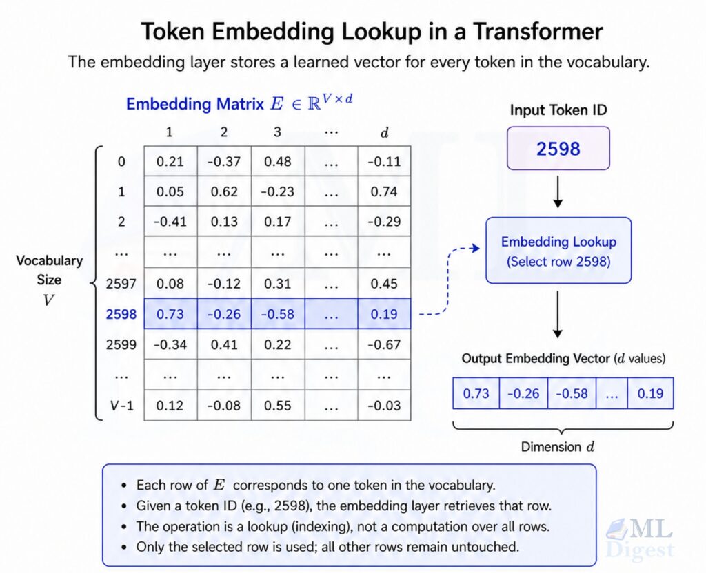
Pooling happens at the output of the encoder, but every transformer also starts with an input embedding step that turns each token ID into an initial vector before any attention is applied. The figure below illustrates that earlier embedding matrix look-up for a single token. More details on the embedding layer are in the embedding layer of Transformer architecture article.
4.4 Bi-encoders, cross-encoders, and late interaction
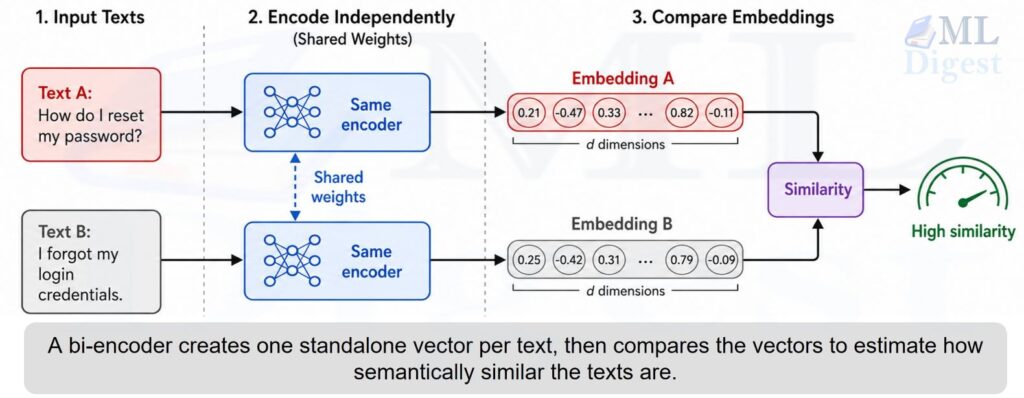
A bi-encoder independently embeds the query and each document. Its vectors can be precomputed and indexed, making it fast enough for first-stage retrieval. Models from Sentence Transformers are common examples.
A cross-encoder receives a query and candidate together, then allows full cross-attention between them. It generally ranks a small candidate set more accurately, but cannot precompute independent document vectors. A practical pattern is therefore retrieve with a bi-encoder, then rerank the top $k$ results with a cross-encoder.
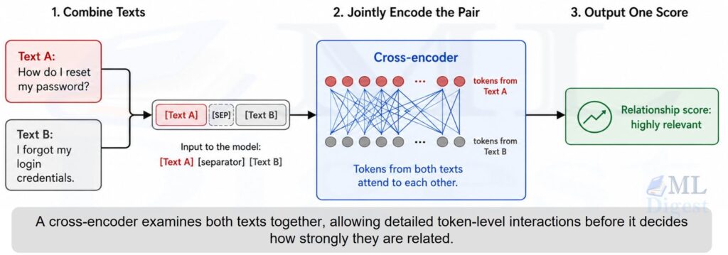
Late-interaction models, such as ColBERT, retain multiple token vectors per document and compare them at token granularity. They offer a quality-latency compromise, but require more storage and a specialized index.
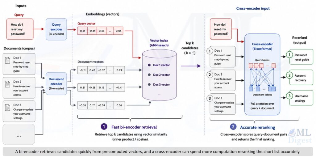
As shown in the figure above, a bi-encoder retrieves candidates quickly from precomputed vectors, and a cross-encoder can spend more computation reranking the short list accurately.
4.5 Embedding-model examples
| Family | Examples | Best fit | Main trade-off |
|---|---|---|---|
| Sparse lexical | TF-IDF, BM25 | Exact terms, transparent baseline, rare identifiers | Weak synonym and paraphrase matching |
| Static dense | Word2Vec, GloVe, fastText | Lightweight word-level features | Context is lost |
| General transformer encoder | BERT, RoBERTa | Fine-tuned classification and token tasks | Raw pooling may be weak for retrieval |
| Sentence or retrieval bi-encoder | all-MiniLM-L6-v2, E5, BGE | Semantic search, clustering, RAG retrieval | Can miss fine-grained relevance |
| Hosted embedding API | OpenAI text-embedding-3 | Managed production workflows | Cost, network dependency, data-governance review |
| Multilingual model | LaBSE, multilingual-e5 | Cross-language retrieval | Quality varies across languages and domains |
5. Dense Embedding Based Document Retrieval
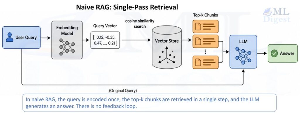
Embeddings power the retrieval layer of a document-search system. This section focuses on the representation and nearest-neighbor search steps: how text becomes comparable vectors, how those vectors are indexed, and how a query finds nearby chunks.
5.1 Chunk documents for embedding
Collect source documents, preserve useful metadata, remove boilerplate, and split text into coherent chunks. A chunk should contain enough context to express one idea, but not so much unrelated content that its vector becomes a semantic average. For detailed guidance, see chunking for retrieval-augmented generation.
5.2 Choose and evaluate the embedding model
Choose a model trained for the actual similarity objective. Query-to-passage retrieval needs a retrieval model, whereas duplicate detection may benefit more from a paraphrase model. Check the maximum input length, output dimension, languages, license, cost, hardware requirements, and any query or document prefixes required by the model card. Some retrieval models use different prefixes for queries and passages, so apply the documented template consistently to each side.
Create a small evaluation set from real queries before committing. For every query, label the chunks a user would consider relevant. Measure Recall@$k$, Mean Reciprocal Rank (MRR), and nDCG, then inspect failures manually.
5.3 Encode, normalize, and index vectors
This runnable Python example creates embeddings locally with Sentence Transformers, normalizes them, and retrieves the most similar chunks.
Sample Code Snippet:
from sentence_transformers import SentenceTransformer
import numpy as np

# A compact general-purpose model. Confirm its license and benchmark it on your data.
model = SentenceTransformer("all-MiniLM-L6-v2")

chunks = [
    "Reset a password from the Account Settings page.",
    "Travel tips for visiting Tokyo in spring.",
    "Account recovery requires access to your verified email address.",
]
query = "I forgot my login password. How can I access my account?"

# normalize_embeddings=True makes dot product equivalent to cosine similarity.
chunk_vectors = model.encode(
    chunks, normalize_embeddings=True, convert_to_numpy=True
)
query_vector = model.encode(
    [query], normalize_embeddings=True, convert_to_numpy=True
)[0]

# Each row is a chunk vector. Larger scores indicate closer semantic matches.
scores = chunk_vectors @ query_vector
ranked_indices = np.argsort(scores)[::-1]

for index in ranked_indices:
print(f"{scores[index]:.3f} {chunks[index]}")For a small corpus, an in-memory matrix is enough. At larger scale, store vectors and metadata in a vector index that supports approximate nearest-neighbor (ANN) search. ANN deliberately trades a small amount of recall for much lower latency.
5.4 Embed queries and retrieve nearest chunks
At search time, apply the same text-cleaning rules, embedding model version, normalization, and model-specific query template used during evaluation. Embed the query, compute its similarity to indexed chunk vectors, and return the top $k$ nearest chunks. Apply metadata and access-control filters as part of retrieval so that only eligible chunks can appear in the result set. The practical details of diagnosing poor retrieval are covered in debugging a RAG workflow.
Log query distributions, similarity-score distributions, clicked or accepted chunks, latency, and failure cases. Re-embed the corpus when the embedding model, text preprocessing, chunking strategy, or normalization changes. Mixing vectors from incompatible representations in one index is a quiet but serious production bug. A reranker may improve a short list later, but it is a separate relevance-modeling step, not part of embedding retrieval itself.
6. Where Text Embeddings Are Used
Document retrieval is only one consumer of the same vectors. Embeddings usually sit behind an application feature rather than appearing directly in the interface, and the techniques from the sections above recur across several other use cases.
- Semantic search and enterprise knowledge assistants: retrieve policy, documentation, support, or code snippets that answer a natural-language question.
- RAG: ground a generator in relevant private or fresh information, reducing the chance that it answers solely from parametric memory. Retrieval still needs evaluation because irrelevant context can harm an answer.
- Recommendations: represent users, products, articles, and queries in compatible spaces to find related items. See recommendation systems for the broader system design.
- Support-ticket routing and intent detection: compare a new ticket to labeled examples, cluster recurring issues, or send it to the right queue.
- Clustering and data exploration: map a large unlabelled corpus into groups. Use k-means clustering cautiously, review groups with humans, and use the silhouette score as one diagnostic rather than trusting coordinates alone. Name groups from their source texts.
- Deduplication, moderation triage, and anomaly investigation: identify near-duplicate records, semantically related reports, or examples unlike known clusters.
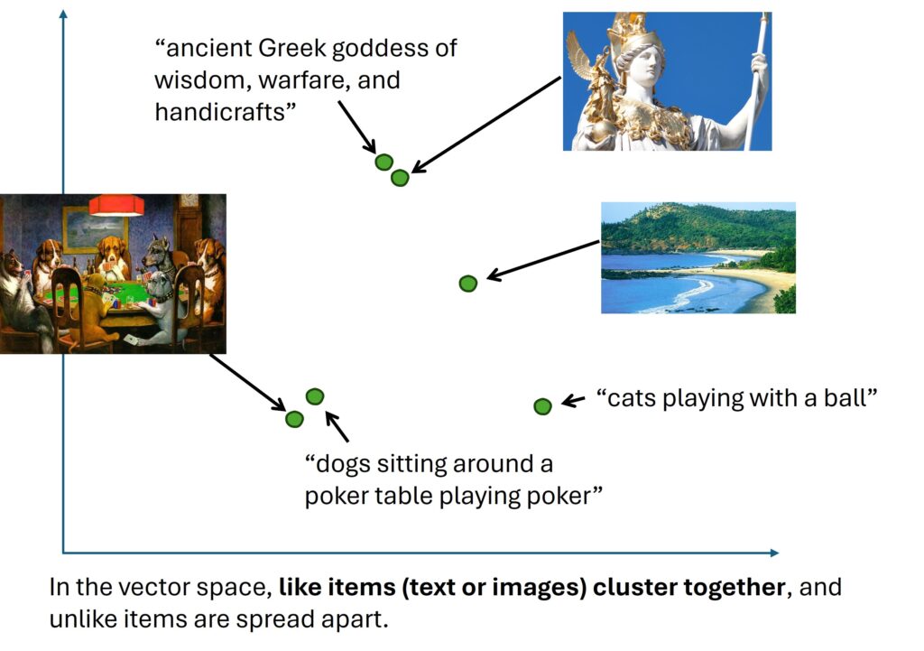
As shown in the figure above, embeddings can also connect text with other modalities. CLIP jointly embeds images and captions into a shared space, so a text query can retrieve relevant images and vice versa.
7. Challenges and Limitations
Despite this broad range of uses, embeddings are not a free lunch. An embedding similarity score is not a truth score. It measures closeness under a particular model, objective, and input distribution. Production systems need safeguards around that fact.
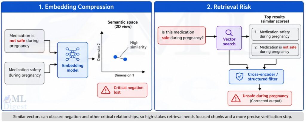
Meaning can be compressed away
One vector must summarize an entire chunk. Important details, negation, quantities, dates, and relationships can vanish. “The medication is not safe during pregnancy” can become dangerously close to text that merely discusses medication safety. Keep chunks focused, retrieve more candidates before reranking, and use a cross-encoder or structured filters when precision is critical.
Domain and language mismatch
A general model may not recognize internal abbreviations, legal concepts, clinical language, new products, or low-resource languages. Benchmark on representative data. If quality remains weak, choose a domain-specific or multilingual model, curate hard-negative training data, or fine-tune a bi-encoder. Do not assume a higher benchmark score transfers to your corpus.
Bias, privacy, and security
Embeddings can preserve social biases in training data and may enable sensitive inferences when combined with other information; see ethics and fairness in machine learning for broader mitigation strategies. Private text sent to a hosted API requires a data-processing and retention review. Apply access filters before exposing retrieved content, encrypt data as appropriate, and test for cross-tenant retrieval leaks. For practical privacy guidance, read protecting privacy in the age of AI; for broader risk-management principles, read responsible AI.
Cost, latency, and index maintenance
Encoding a large corpus costs time and compute. High-dimensional vectors consume storage and memory, while ANN indexes have parameters that change recall and latency. Version every model and index, set re-embedding procedures, track cost per document and query, and use batching for throughput. Smaller models can be the best choice when they meet the measured quality target.
Evaluation is often too narrow
Offline retrieval metrics may hide failure modes for rare intents, long queries, multilingual queries, or adversarial wording. Build a test set from production logs, slice results by user group and topic, and review errors with domain experts. Measure the end-to-end outcome, such as successful support resolution, not only nearest-neighbor accuracy.
Summary
Text embeddings turn language into vectors whose relative positions capture useful semantic relationships. Traditional TF-IDF and BM25 remain valuable lexical baselines, static word vectors offer efficient word-level features, and transformer bi-encoders enable powerful modern semantic retrieval. The model is only one piece of the system: chunking, similarity metrics, indexing, permissions, reranking, and evaluation determine whether embeddings help real users.
Start small: embed a representative document collection, compare a dense model against BM25 on 20 to 50 real queries, and inspect every surprising result. Then use the evidence to tune chunking, select a model, and build a retrieval pipeline that earns its place in production.

Happy is a seasoned ML professional with over 15 years of experience. His expertise spans various domains, including Computer Vision, Natural Language Processing (NLP), and Time Series analysis. He holds a PhD in Machine Learning from IIT Kharagpur and has furthered his research with postdoctoral experience at INRIA-Sophia Antipolis, France. Happy has a proven track record of delivering impactful ML solutions to clients. Check more about him here: https://sites.google.com/site/slhappyin/

Silpa brings 5 years of experience in working on diverse ML projects, specializing in designing end-to-end ML systems tailored for real-time applications. Her background in statistics (Bachelor of Technology) provides a strong foundation for her work in the field. Silpa is also the driving force behind the development of the content you find on this site.
Subscribe to our newsletter!