Imagine you are trying to recognize a cat in a photograph. You do not scan the entire image at once. Instead, your eyes naturally zero in on local clues: the pointed ears, the whisker lines, the slitted pupils. You combine those local clues into mid-level features (a furry face with ears), and eventually arrive at the conclusion: “That is a cat.”
This is, in essence, what a Convolutional Neural Network (CNN) does. It processes an image progressively, building up from tiny local patterns (edges, corners, textures) to larger structures (eyes, noses) to full objects, layer by layer. Unlike a fully connected network, which treats every pixel as an independent input, a CNN exploits two powerful facts about images:
- Local structure matters. Pixels that are close together are more related than pixels that are far apart.
- Patterns repeat. The edge detector that finds a cat’s ear works just as well at the top-left of the image as at the bottom-right. There is no need to learn a separate detector for every position.
These two ideas, local connectivity and weight sharing, are the DNA of CNNs. Introduced in their modern form by LeCun et al. in 1989 and popularized for deep learning by AlexNet in 2012, CNNs became the backbone of computer vision research for over a decade and remain one of the most important tools in the field today.
1. The Convolution Operation
1.1 What is a Convolution?
Start with a simple picture. You have a grayscale image, a grid of numbers where each number represents the brightness of one pixel. You also have a small grid of numbers, say 3×3, called a kernel (or filter). The kernel slides across the image, and at every position, you multiply each kernel weight by the corresponding pixel value underneath it, then sum all the products into a single number. That number becomes one value in the output feature map.
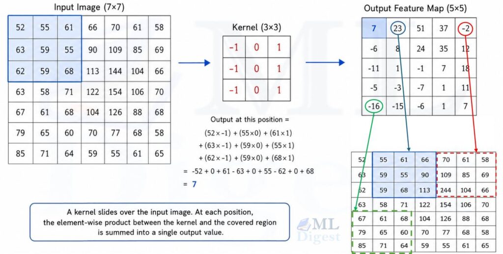
Formally, for a 2D input $I$ and a kernel $K$ of size $k \times k$, the output feature map $S$ at position $(i, j)$ is:
$$
S(i, j) = \sum_{m=0}^{k-1} \sum_{n=0}^{k-1} I(i+m,\; j+n) \cdot K(m, n)
$$
This is technically a cross-correlation rather than a strict mathematical convolution (which would flip the kernel), but the two are equivalent in practice because the kernel weights are learned and can absorb any flip. The deep learning community universally calls this operation “convolution.”
1.2 What Does a Kernel Learn?
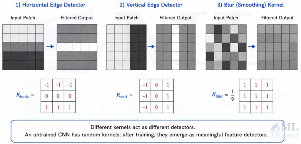
Different kernels detect different patterns. A kernel that looks like this:
$$
K_{\text{horiz}} = \begin{bmatrix} -1 & -1 & -1 \\ 0 & 0 & 0 \\ 1 & 1 & 1 \end{bmatrix}
$$
is a horizontal edge detector. More precisely, it responds strongly to a horizontal intensity transition: with the sign convention above, it produces a positive response when pixels below are brighter than pixels above, and a negative response for the opposite transition. The beauty of CNNs is that kernels like this are not hand-designed. The network learns them from data during training.
1.3 Extending to Color Images and Multiple Filters
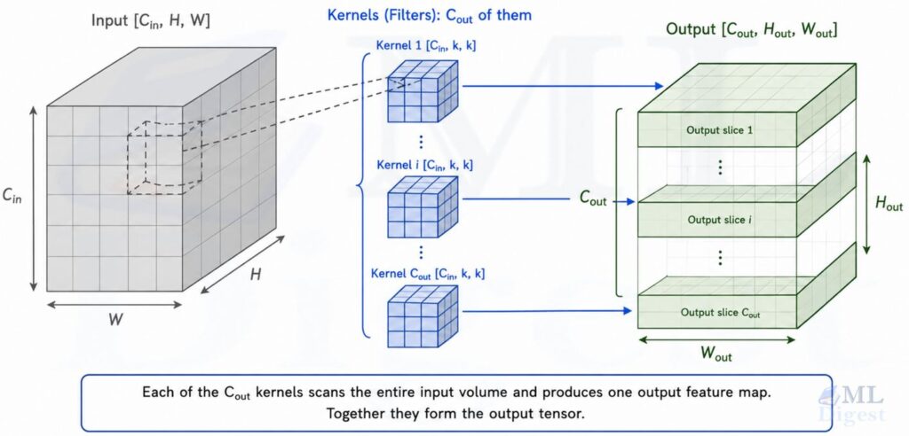
Real images have three channels: Red, Green, and Blue. The kernel extends into a volume: for an input with $C_{\text{in}}$ channels, the kernel has shape $C_{\text{in}} \times k \times k$. The operation sums over all input channels, still producing a single scalar per spatial position:
$$
S(i, j) = \sum_{c=0}^{C_{\text{in}}-1} \sum_{m=0}^{k-1} \sum_{n=0}^{k-1} I(c,\; i+m,\; j+n) \cdot K(c,\; m,\; n) + b
$$
where $b$ is a learned bias term.
A single kernel produces one output feature map. To detect multiple different patterns, the layer uses $C_{\text{out}}$ independent kernels, each producing its own feature map. The full output is a volume of shape $C_{\text{out}} \times H_{\text{out}} \times W_{\text{out}}$, often called a tensor.
1.4 Stride and Padding
Two hyperparameters control the geometry of the convolution:
Stride ($s$): the step size of the sliding window. With stride 1, the kernel moves one pixel at a time. With stride 2, it jumps two pixels, halving the spatial dimensions of the output. The output size is:
$$
H_{\text{out}} = \left\lfloor \frac{H_{\text{in}} – k + 2p}{s} \right\rfloor + 1
$$
where $p$ is the padding.
Padding ($p$): zero-valued pixels added around the border of the input. Without padding, the output is smaller than the input (a 3×3 kernel applied with no padding shrinks a 7×7 input to a 5×5 output). For odd-sized kernels, same padding typically means $p = (k-1)/2$, which preserves the spatial size when stride is 1.
A practical rule of thumb: use same padding and stride 1 for most convolutions, and use stride 2 (or a pooling layer) when you want to downsample.
2. Pooling Layers
After a convolution, the network often applies a pooling layer to reduce the spatial size of the feature map. This reduces the number of activations and computations in subsequent layers, and it introduces a limited degree of spatial invariance, since the response is preserved even if the detected pattern shifts slightly.
The most common variant is max pooling: a small window (typically 2×2) slides over the feature map with a stride equal to its size, and the maximum value in each window becomes the output.
$$
\text{MaxPool}(i, j) = \max_{0 \le m < k,\; 0 \le n < k} S(i \cdot s + m,\; j \cdot s + n)
$$
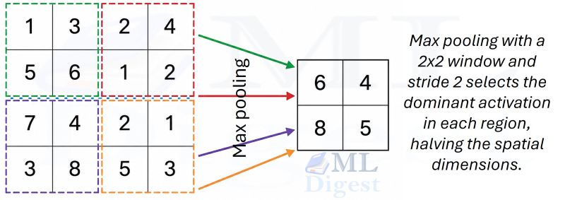
Average pooling computes the mean instead of the maximum. In modern architectures, global average pooling (GAP) reduces an entire feature map to a single number per channel by averaging all spatial positions. It is widely used as the last step before the classification head, replacing the large fully connected layers of older architectures.
3. Activation Functions
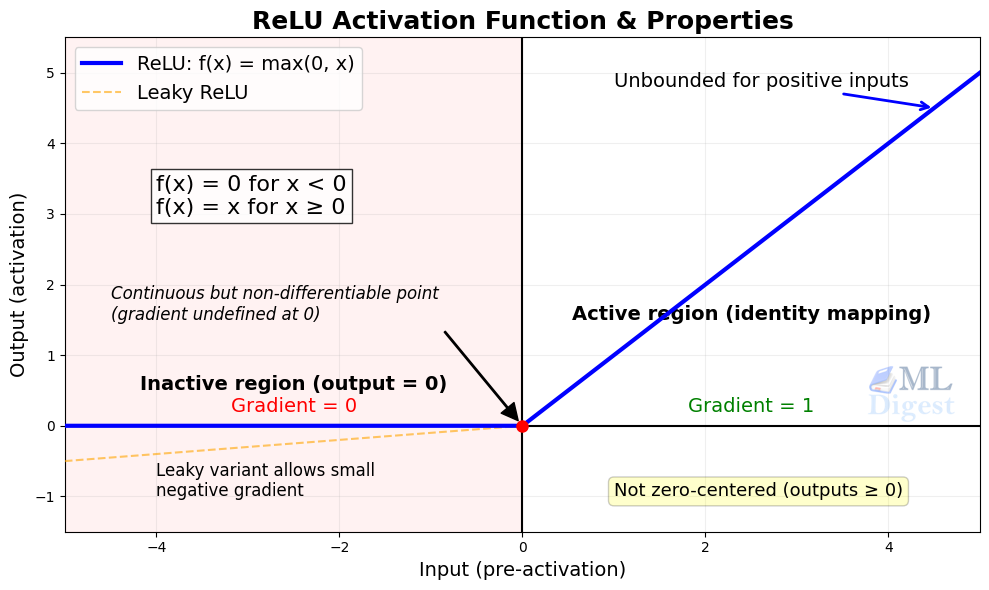
A stack of convolutions is still linear until a nonlinearity is inserted. Without it, multiple convolution layers collapse into a single linear transformation, no richer than one layer. Pooling can shrink spatial dimensions, but it is not a substitute for a learned activation function. An activation function applied after each convolution introduces the nonlinearity that allows the network to learn complex, curved decision boundaries.
The standard choice is the Rectified Linear Unit (ReLU):
$$
\text{ReLU}(x) = \max(0, x)
$$
It is computationally cheap, has a non-saturating gradient for positive inputs (helping address the vanishing gradient problem that plagued sigmoid and tanh activations in deep networks), and works remarkably well in practice. Modern networks sometimes use variants such as Leaky ReLU (which allows a small gradient for negative inputs) or GELU (used in Transformers and some modern CNNs).
4. Putting It All Together: The CNN Architecture
A complete CNN chains these building blocks into a two-stage structure:
- Feature extraction backbone: alternating convolution, activation, and pooling layers that transform the raw image into a rich abstract representation.
- Classification head: one or more fully connected (linear) layers that map the abstract representation to class scores.

4.1 The Receptive Field
One of the most important concepts for understanding how CNNs process information is the receptive field: the region of the original input image that influences a single neuron in a given layer.
A single neuron in the first conv layer (with a 3×3 kernel) sees a 3×3 region of the input. A neuron in the second conv layer sees a 3×3 region of the first conv layer’s output, which itself covered a 5×5 region of the input. Each layer stacks on top of the last, and the receptive field grows:
- After 1 conv layer (3×3 kernel): receptive field = 3×3
- After 2 conv layers: 5×5
- After 3 conv layers: 7×7
For a stack of $L$ stride-1 convolutions with kernel size $k$ and no dilation, the receptive field grows as $1 + L \cdot (k – 1)$. Pooling layers, strided convolutions, and dilation increase the effective receptive field more quickly, so the exact growth depends on the full stack of kernels, strides, paddings, and dilation rates.
This explains why deeper networks can recognize large objects: their later layers have receptive fields that span most of the image.
4.2 Channel Depth Increases, Spatial Size Decreases
As the spatial dimensions shrink through pooling or strided convolutions, the number of channels typically grows. This is a deliberate design choice. Early layers detect many types of simple local patterns, so many channels are useful even though the feature maps are large. Later layers operate on smaller spatial grids, but with richer, more abstract channels. In practice, architectures trade spatial resolution for channel depth to preserve representational power as tensors get smaller.
5. Training CNNs: Backpropagation Through Convolutions
A CNN is trained like any neural network: using stochastic gradient descent (SGD) or an adaptive optimizer (Adam, AdamW) to minimize a loss function (typically cross-entropy for classification). Gradients flow backward through each layer via backpropagation.
The gradient of the loss with respect to a kernel weight $K(m, n)$ is:
$$
\frac{\partial \mathcal{L}}{\partial K(m, n)} = \sum_{i} \sum_{j} \frac{\partial \mathcal{L}}{\partial S(i, j)} \cdot I(i+m,\; j+n)
$$
This is another cross-correlation: the gradient with respect to a kernel is the cross-correlation of the incoming gradient with the input. The same kernel is reused at many positions, so the gradient accumulates contributions from all of them. This is exactly the gradient of the shared weights.
For the gradient with respect to the input (needed to continue backpropagation into earlier layers), the operation is a full convolution of the incoming gradient with the flipped kernel. The key point for practitioners is that modern frameworks such as PyTorch and TensorFlow handle all of this automatically.
5.1 Regularization in CNNs
Training a deep CNN on a limited dataset without regularization leads to overfitting. The standard toolkit overlaps heavily with the broader set of regularization techniques in neural networks, but a few methods are especially common in vision:
- Dropout: randomly zeroes a fraction of activations during training. Applied after fully connected layers.
- Batch Normalization: normalizes each feature map to zero mean and unit variance within a mini-batch, then applies learned scale and shift parameters. This stabilizes training, allows higher learning rates, and acts as a mild regularizer.
- Data augmentation: randomly flip, crop, rotate, or color-jitter training images to artificially expand the dataset and force the model to learn invariances.
- Weight decay: L2 regularization on the kernel weights, penalizing large values.
6. A Brief History of CNN Architectures
Understanding how architectures evolved gives insight into the design decisions that are now standard practice.
6.1 LeNet-5 (1998)
LeNet-5 (LeCun et al.) was the first practical CNN, designed to read handwritten digits on cheques. It had only 60,000 parameters: two convolutional layers followed by average pooling, and three fully connected layers. On a 32×32 input, it achieved near-human accuracy on MNIST. Its core idea, local filters and weight sharing, remains unchanged in today’s architectures.
6.2 AlexNet (2012)
AlexNet (Krizhevsky, Sutskever, and Hinton) won the ImageNet Large Scale Visual Recognition Challenge (ILSVRC) in 2012 by a margin of over 10 percentage points, igniting the modern deep learning era. Its key contributions were:
- ReLU activations instead of tanh, enabling faster training of deeper networks.
- Training on GPUs, making it possible to handle millions of parameters.
- Dropout for regularization.
- Data augmentation (random crops and horizontal flips).
With 60 million parameters and five convolutional layers, AlexNet demonstrated that scale and GPUs together could push well beyond hand-crafted feature pipelines.
6.3 VGGNet (2014)
VGGNet (Simonyan and Zisserman) made the bold architectural claim that depth, using only 3×3 kernels, was the key driver of performance. Two stacked 3×3 convolutions have the same receptive field as one 5×5 convolution but fewer parameters ($2 \times 9 C^2$ vs. $25 C^2$) and an extra nonlinearity. VGG-16 (16 weight layers) and VGG-19 became standard baselines and showed that going deeper with small kernels systematically improved accuracy.
6.4 ResNet (2015)
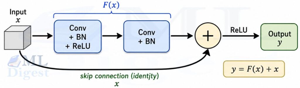
ResNet solved the degradation problem: simply stacking more layers eventually made training worse, not because of overfitting but because gradients vanished in very deep networks. The solution was the residual connection (skip connection): the output of a block is $F(x) + x$ instead of just $F(x)$.
$$
\text{output} = F(x, {W_i}) + x
$$
If the optimal transformation at a layer is close to the identity, the residual block can simply drive $F(x)$ toward zero. The skip connection provides a direct path for gradients to flow backward through dozens or hundreds of layers. ResNet-50 and ResNet-101 became the go-to backbones for transfer learning for years, and residual connections are now a nearly universal component of modern architectures.
7. Implementation in PyTorch
Click to expand and see the python implementation
7.1 Building a Simple CNN from Scratch
This example builds a small but complete CNN for classifying 32×32 RGB images into 10 classes (the CIFAR-10 format).
import torch
import torch.nn as nn
import torch.nn.functional as F


class SimpleCNN(nn.Module):
    """
    A small convolutional network for 32x32 RGB image classification.
    Architecture: Conv -> BN -> ReLU -> Pool (repeated), then GAP + Linear.
    """

    def __init__(self, num_classes: int = 10) -> None:
        super().__init__()

        # Stage 1: 3x32x32 -> 32x16x16
        self.stage1 = nn.Sequential(
            nn.Conv2d(in_channels=3, out_channels=32, kernel_size=3, padding=1),
            nn.BatchNorm2d(32),
            nn.ReLU(inplace=True),
            nn.MaxPool2d(kernel_size=2, stride=2),  # halves spatial size
        )

        # Stage 2: 32x16x16 -> 64x8x8
        self.stage2 = nn.Sequential(
            nn.Conv2d(in_channels=32, out_channels=64, kernel_size=3, padding=1),
            nn.BatchNorm2d(64),
            nn.ReLU(inplace=True),
            nn.MaxPool2d(kernel_size=2, stride=2),
        )

        # Stage 3: 64x8x8 -> 128x4x4
        self.stage3 = nn.Sequential(
            nn.Conv2d(in_channels=64, out_channels=128, kernel_size=3, padding=1),
            nn.BatchNorm2d(128),
            nn.ReLU(inplace=True),
            nn.MaxPool2d(kernel_size=2, stride=2),
        )

        # Global average pooling collapses each feature map to a single value
        self.gap = nn.AdaptiveAvgPool2d(output_size=1)  # 128x4x4 -> 128x1x1

        # Classifier head
        self.classifier = nn.Sequential(
            nn.Dropout(p=0.5),
            nn.Linear(128, num_classes),
        )

    def forward(self, x: torch.Tensor) -> torch.Tensor:
        # x: [B, 3, 32, 32]
        x = self.stage1(x)   # [B, 32, 16, 16]
        x = self.stage2(x)   # [B, 64, 8, 8]
        x = self.stage3(x)   # [B, 128, 4, 4]
        x = self.gap(x)      # [B, 128, 1, 1]
        x = x.flatten(1)     # [B, 128]
        x = self.classifier(x)  # [B, num_classes]
        return x


def count_parameters(model: nn.Module) -> int:
    return sum(p.numel() for p in model.parameters() if p.requires_grad)


if __name__ == "__main__":
    model = SimpleCNN(num_classes=10)
    print(f"Trainable parameters: {count_parameters(model):,}")

    # Verify forward pass shapes
    x = torch.randn(4, 3, 32, 32)  # batch of 4 images
    logits = model(x)
    print(f"Input shape:  {x.shape}")
    print(f"Output shape: {logits.shape}")  # expected: [4, 10]
# Expected output:
#     Trainable parameters: 94,986
#     Input shape:  torch.Size([4, 3, 32, 32])
# Output shape: torch.Size([4, 10])7.2 A Minimal ResNet-Style Block
Adding residual connections is straightforward in PyTorch. Here is a self-contained residual block that handles the case where the input and output channel counts differ (using a 1×1 projection shortcut):
import torch
import torch.nn as nn


class ResidualBlock(nn.Module):
    """
    A basic residual block following He et al. (2015).
    Handles shape mismatch via a 1x1 projection shortcut.
    """

    def __init__(
        self,
        in_channels: int,
        out_channels: int,
        stride: int = 1,
    ) -> None:
        super().__init__()

        self.conv_path = nn.Sequential(
            nn.Conv2d(
                in_channels, out_channels,
                kernel_size=3, stride=stride, padding=1, bias=False
            ),
            nn.BatchNorm2d(out_channels),
            nn.ReLU(inplace=True),
            nn.Conv2d(
                out_channels, out_channels,
                kernel_size=3, stride=1, padding=1, bias=False
            ),
            nn.BatchNorm2d(out_channels),
        )

        # If shapes mismatch, project the skip connection to match
        self.shortcut = nn.Identity()
        if stride != 1 or in_channels != out_channels:
            self.shortcut = nn.Sequential(
                nn.Conv2d(
                    in_channels, out_channels,
                    kernel_size=1, stride=stride, bias=False
                ),
                nn.BatchNorm2d(out_channels),
            )

        self.relu = nn.ReLU(inplace=True)

    def forward(self, x: torch.Tensor) -> torch.Tensor:
        return self.relu(self.conv_path(x) + self.shortcut(x))


if __name__ == "__main__":
    # Normal block: same dimensions
    block = ResidualBlock(in_channels=64, out_channels=64)
    x = torch.randn(2, 64, 16, 16)
    print(block(x).shape)  # [2, 64, 16, 16]

    # Downsampling block: stride=2, doubles channels
    block_down = ResidualBlock(in_channels=64, out_channels=128, stride=2)
    print(block_down(x).shape)  # [2, 128, 8, 8]
# Expected output:
#     torch.Size([2, 64, 16, 16])
# torch.Size([2, 128, 8, 8])7.3 Training on CIFAR-10
This complete training loop uses the SimpleCNN above on the CIFAR-10 dataset, which ships with torchvision.
import torch
import torch.nn as nn
import torchvision
import torchvision.transforms as transforms
from torch.utils.data import DataLoader


def get_cifar10_loaders(batch_size: int = 128) -> tuple[DataLoader, DataLoader]:
    # Training augmentation: random horizontal flip and random crop
    train_transform = transforms.Compose([
        transforms.RandomHorizontalFlip(),
        transforms.RandomCrop(32, padding=4),
        transforms.ToTensor(),
        transforms.Normalize(
            mean=[0.4914, 0.4822, 0.4465],
            std=[0.2470, 0.2435, 0.2616],
        ),
    ])
    val_transform = transforms.Compose([
        transforms.ToTensor(),
        transforms.Normalize(
            mean=[0.4914, 0.4822, 0.4465],
            std=[0.2470, 0.2435, 0.2616],
        ),
    ])

    train_ds = torchvision.datasets.CIFAR10(
        root="./data", train=True, download=True, transform=train_transform
    )
    val_ds = torchvision.datasets.CIFAR10(
        root="./data", train=False, download=True, transform=val_transform
    )
    train_loader = DataLoader(train_ds, batch_size=batch_size, shuffle=True, num_workers=4)
    val_loader = DataLoader(val_ds, batch_size=batch_size, shuffle=False, num_workers=4)
    return train_loader, val_loader


def train_one_epoch(
    model: nn.Module,
    loader: DataLoader,
    optimizer: torch.optim.Optimizer,
    criterion: nn.Module,
    device: torch.device,
) -> float:
    model.train()
    total_loss = 0.0
    for images, labels in loader:
        images, labels = images.to(device), labels.to(device)
        optimizer.zero_grad()
        logits = model(images)
        loss = criterion(logits, labels)
        loss.backward()
        optimizer.step()
        total_loss += loss.item() * images.size(0)
    return total_loss / len(loader.dataset)


@torch.inference_mode()
def evaluate(
    model: nn.Module,
    loader: DataLoader,
    device: torch.device,
) -> float:
    model.eval()
    correct = 0
    for images, labels in loader:
        images, labels = images.to(device), labels.to(device)
        preds = model(images).argmax(dim=1)
        correct += (preds == labels).sum().item()
    return correct / len(loader.dataset)


def main() -> None:
    device = torch.device("cuda" if torch.cuda.is_available() else "cpu")
    print(f"Using device: {device}")

    train_loader, val_loader = get_cifar10_loaders(batch_size=128)

    model = SimpleCNN(num_classes=10).to(device)
    criterion = nn.CrossEntropyLoss()
    optimizer = torch.optim.AdamW(model.parameters(), lr=1e-3, weight_decay=1e-4)
    scheduler = torch.optim.lr_scheduler.CosineAnnealingLR(optimizer, T_max=30)

    for epoch in range(1, 31):
        train_loss = train_one_epoch(model, train_loader, optimizer, criterion, device)
        val_acc = evaluate(model, val_loader, device)
        scheduler.step()
        print(f"Epoch {epoch:02d} | Loss: {train_loss:.4f} | Val Acc: {val_acc:.4f}")


if __name__ == "__main__":
main()With this setup and 30 epochs, SimpleCNN typically reaches around 80-82% validation accuracy on CIFAR-10, which is a solid baseline for a network this small.
8. Practical Tips and Best Practices
8.1 Use Pretrained Models for Transfer Learning
Training a CNN from scratch often benefits from large datasets and significant compute. For most practical problems, transfer learning from a network pretrained on ImageNet is a better starting point than random initialization. Libraries like timm and torchvision.models provide access to dozens of pretrained architectures.
The standard recipe:
- Load a pretrained backbone (ResNet-50, EfficientNet-B0, ConvNeXt, etc.).
- Replace the final classification head with a new
nn.Linear(in_features, num_classes). - Freeze the backbone and train only the head for a few epochs.
- Unfreeze the full model and fine-tune end-to-end with a small learning rate ($10^{-4}$ or lower).
8.2 Data Augmentation is Essential
The single most impactful regularization technique for CNNs is data augmentation. Even simple augmentations (random horizontal flip, random crop with padding) can push accuracy up by several percentage points. For tougher problems, consider:
- RandAugment: a policy that randomly selects from a large set of augmentation operations.
- Mixup: linearly interpolates between two training images and their labels.
- CutMix: replaces a random rectangular region of one image with a patch from another.
8.3 Batch Normalization is a Default Ingredient
Almost every modern CNN uses Batch Normalization after each convolution. It keeps activations in a reasonable range throughout training, reduces sensitivity to weight initialization, and allows the use of higher learning rates. Always place it before the activation function (Conv -> BN -> ReLU).
There is one important caveat: Batch Normalization behaves differently during training and inference. Always call model.train() during training and model.eval() during evaluation. Forgetting this is one of the most common bugs in CNN training.
8.4 Choose Kernel Size 3×3 as the Default
VGGNet demonstrated empirically that stacking 3×3 kernels is more parameter-efficient than using larger kernels. Two 3×3 convolutions cover the same 5×5 receptive field as one 5×5 convolution but with fewer parameters ($2 \times 9 C^2 = 18C^2$ vs. $25C^2$) and an extra nonlinearity. Stick with 3×3 for most convolutions. Larger kernels (5×5 or 7×7) are sometimes used only in the very first layer to process the input image.
8.5 Match Input Normalization to the Pretrained Model
When using pretrained weights, the input image should be preprocessed with the same pipeline used during pretraining. For many ImageNet-pretrained models that includes normalization close to the familiar ImageNet mean and standard deviation values below, but resize, crop, and interpolation details can also matter:
transforms.Normalize(mean=[0.485, 0.456, 0.406], std=[0.229, 0.224, 0.225])Using the wrong preprocessing is a silent bug: the model will still run but accuracy can degrade noticeably. In torchvision, prefer the preprocessing attached to the weights object when it is available.
8.6 Learning Rate Scheduling
CNNs benefit greatly from a learning rate schedule. Common choices:
- Cosine annealing: smoothly decays the learning rate from the initial value to near zero over the training run. Works well as a default.
- Step decay: drops the learning rate by a fixed factor (e.g., 0.1) at predefined epochs. Simpler but less smooth.
- Warmup + decay: ramps the learning rate up linearly for the first few epochs (to avoid unstable early updates), then decays it. Especially useful when training from scratch with a large batch size.
If optimization still becomes unstable, gradient clipping is a useful fallback, especially for deeper models or aggressive training settings.
9. Beyond Standard Convolutions
As CNN research matured, several variants of the convolution operation emerged that improve efficiency or expressiveness.
9.1 Depthwise Separable Convolutions
A standard convolution mixes information across both spatial dimensions and channels simultaneously. A depthwise separable convolution, introduced by Chollet in Xception and popularized by MobileNet, splits this into two steps:
- Depthwise convolution: apply a separate spatial filter to each input channel independently (no channel mixing).
- Pointwise convolution: apply a 1×1 convolution to mix the channels.
The compute savings are substantial. For a $k \times k$ kernel with $C$ input channels and $C$ output channels, a standard convolution requires $k^2 C^2$ multiplications per output position, while a depthwise separable convolution requires only $k^2 C + C^2$ (the depthwise step is $k^2 C$, and the pointwise step is $C^2$). This makes it ideal for mobile and embedded applications where efficiency is critical.
9.2 Dilated (Atrous) Convolutions
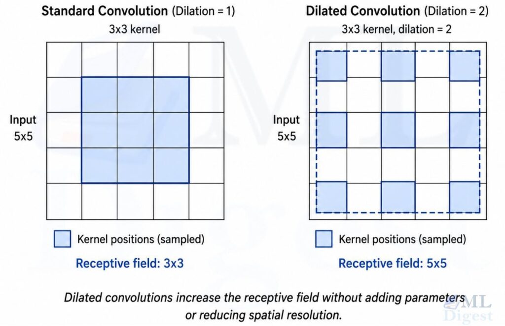
A dilated convolution inserts gaps between kernel elements, allowing the filter to cover a larger area without increasing parameters or stride. The dilation rate $d$ controls the spacing. At $d=2$, a 3×3 kernel covers a 5×5 area; at $d=4$, it covers a 9×9 area.
$$
S(i, j) = \sum_{m} \sum_{n} I(i + d \cdot m,\; j + d \cdot n) \cdot K(m, n)
$$
This is particularly valuable for semantic segmentation, where downsampling via stride or pooling would lose spatial precision needed for pixel-level predictions. DeepLab uses dilated convolutions extensively for this purpose.
Summary
CNNs are built on two elegant ideas: learn local patterns with shared weights, and build up from simple patterns to complex ones by stacking layers. The convolution operation extracts features; pooling compresses them; activation functions introduce the nonlinearity needed for complex decisions; and residual connections allow gradients to flow through hundreds of layers.
Here are the key takeaways:
- A kernel is a small learnable filter. It slides across the input and detects one type of pattern at any position.
- Feature maps capture multiple types of patterns simultaneously. With $C_{\text{out}}$ kernels, the output has $C_{\text{out}}$ channels.
- Pooling reduces spatial size and introduces limited invariance to small translations.
- CNNs alternate between growing channel depth and reducing spatial size, converting an image into a compact vector.
- Residual connections made it practical to train very deep networks by providing a gradient highway.
- For applied work, transfer learning from ImageNet-pretrained backbones dramatically outperforms training from scratch on most datasets.
The best way to build intuition is to train one yourself. Start with the CIFAR-10 example above, inspect the learned kernels in the first layer (they typically look like oriented edge detectors after training), and experiment with adding residual blocks. From there, the jump to modern architectures like ResNet, EfficientNet, Vision Transformers, DETR, or ConvNeXt is a series of principled engineering improvements on the same foundation.

Silpa brings 5 years of experience in working on diverse ML projects, specializing in designing end-to-end ML systems tailored for real-time applications. Her background in statistics (Bachelor of Technology) provides a strong foundation for her work in the field. Silpa is also the driving force behind the development of the content you find on this site.

Happy is a seasoned ML professional with over 15 years of experience. His expertise spans various domains, including Computer Vision, Natural Language Processing (NLP), and Time Series analysis. He holds a PhD in Machine Learning from IIT Kharagpur and has furthered his research with postdoctoral experience at INRIA-Sophia Antipolis, France. Happy has a proven track record of delivering impactful ML solutions to clients. Check more about him here: https://sites.google.com/site/slhappyin/
Subscribe to our newsletter!