When you read the fragment, “She reached into her bag and pulled out a …”, your mind immediately narrows the possibilities. You are not solving a formal optimization problem. You are using patterns absorbed from books, articles, conversations, and lived experience to predict what is likely to come next.
GPT applies the same basic idea at machine scale. It learns to predict the next token in a sequence, over and over, across massive text corpora. That objective looks narrow, but at sufficient scale it produces representations that capture syntax, style, factual associations, and many useful reasoning patterns. This article explains the key pieces behind that result: tokenization, causal language modeling, the decoder-only Transformer architecture, the training pipeline, and the progression from GPT-1 to GPT-4.
1. What GPT Is (and Is Not)
GPT stands for Generative Pre-trained Transformer. Each term matters:
- Generative means the model produces new text token by token, rather than only assigning labels or extracting spans from an input.
- Pre-trained means the model is first trained on a broad corpus and only later adapted, aligned, or specialized for downstream use.
- Transformer refers to the neural architecture introduced in Attention Is All You Need by Vaswani et al. (2017). If you want the broader architectural background first, see this overview of the Transformer model.
It is also useful to clarify what GPT is not. The original Transformer contains an encoder and a decoder. GPT keeps only the decoder stack. That design choice fits the objective: for left-to-right text generation, the model only needs access to the tokens that have already appeared. There is no separate source sequence to encode, so the encoder and encoder-decoder cross-attention are unnecessary.
2. Before the Model: Text Becomes Tokens
GPT does not read raw characters or whole words directly. It reads tokens, compact units produced by a tokenizer. Many GPT-style models use subword tokenization schemes in the BPE family. For example, GPT-2 and GPT-3 use byte-level BPE, which splits text into reusable pieces such as word fragments, punctuation, and whitespace patterns while still being able to represent arbitrary byte sequences. If you want the tokenization mechanism itself unpacked, see Byte Pair Encoding (BPE).
That detail matters for three reasons:
- The model predicts the next token, not necessarily the next word.
- The context window is measured in tokens, so tokenization affects how much text the model can process at once.
- Rare words can still be represented compositionally, because they can be broken into smaller known pieces.
3. The Core Learning Objective
GPT is trained with the causal language modeling objective: given tokens $x_1, x_2, \ldots, x_{t-1}$, predict token $x_t$.
Formally, the model maximizes the log-likelihood over a corpus $\mathcal{D}$ of token sequences:
$$\mathcal{L} = \sum_i \sum_t \log P\left(x_t^{(i)} \mid x_1^{(i)}, \ldots, x_{t-1}^{(i)}; \theta\right)$$
where $\theta$ denotes the model parameters.
This is a classic form of self-supervision. No one has to label documents by hand. Every sequence already contains its own training signal, because each token serves as the target for the previous context. Books, web pages, code, and articles become supervision automatically.
This setup differs from BERT, which uses masked language modeling and can look in both directions around a masked token. GPT is strictly left-to-right during training, which makes it naturally suited for generation.
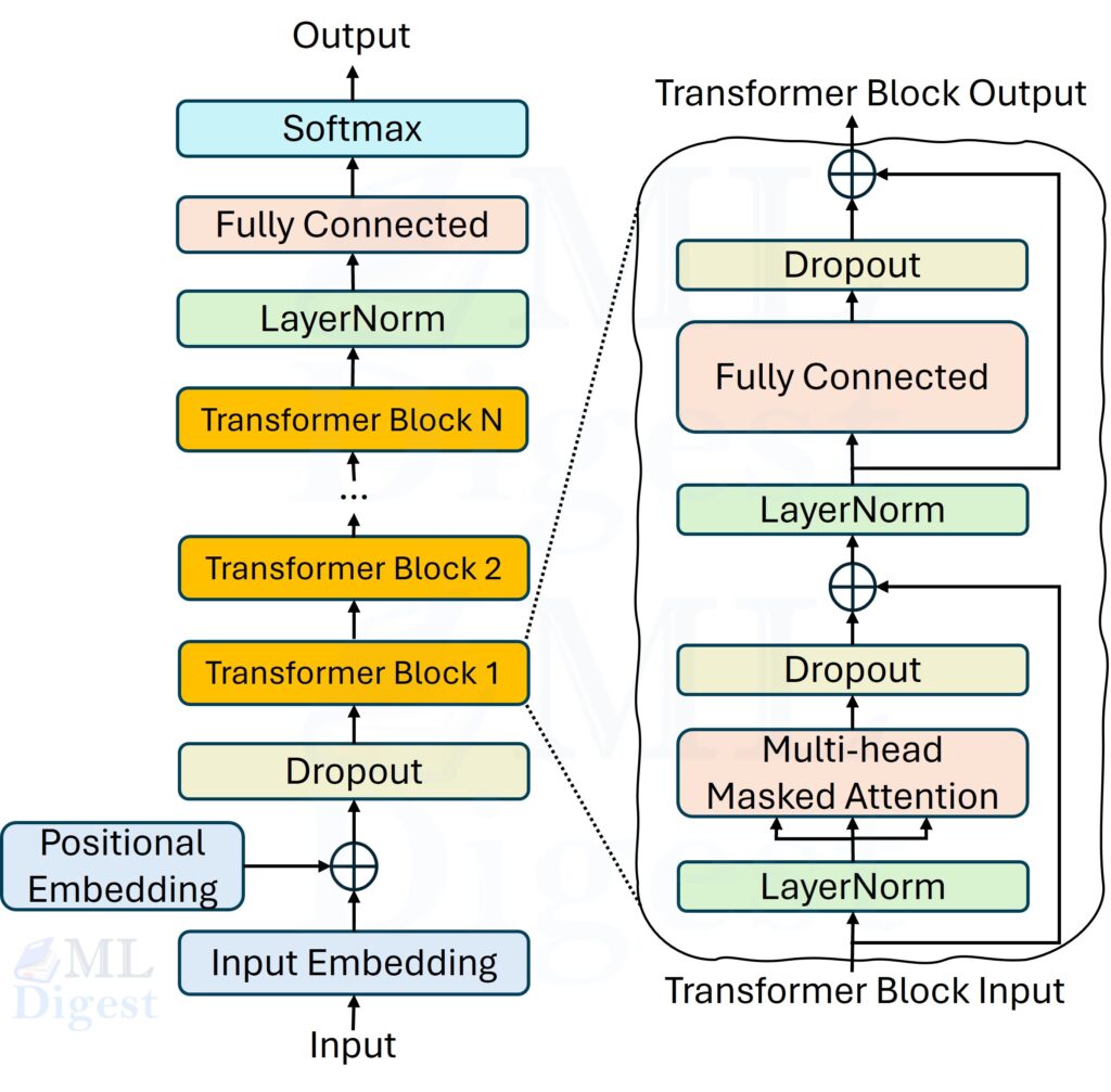
4. Architecture: The Decoder-Only Transformer
4.1 High-Level Overview
Each GPT model is a stack of $N$ transformer decoder blocks. Each block contains two main sub-layers:
- masked multi-head self-attention
- a position-wise feed-forward network
These sub-layers are wrapped with residual connections and layer normalization. Many practical GPT implementations also include dropout during training.
4.2 Input Representation
The input sequence is first converted into token indices. Each index is mapped to a learned embedding vector $e_t \in \mathbb{R}^d$ through a token embedding matrix $W_E \in \mathbb{R}^{|\mathcal{V}| \times d}$, where $|\mathcal{V}|$ is the vocabulary size and $d$ is the model dimension. For more detail on how token vectors are learned and used, see architecture and training of the embedding layer of LLMs.
Since the self-attention operation itself is permutation-equivariant (it has no built-in notion of order), positional information must be injected explicitly. GPT uses a learned positional embedding $p_t \in \mathbb{R}^d$, so the input representation for position $t$ is simply:
$$h_t^{(0)} = e_t + p_t$$
This sum gives the model both token identity and position information.
Other architectures use different schemes, which we discuss in absolute vs relative position embeddings.
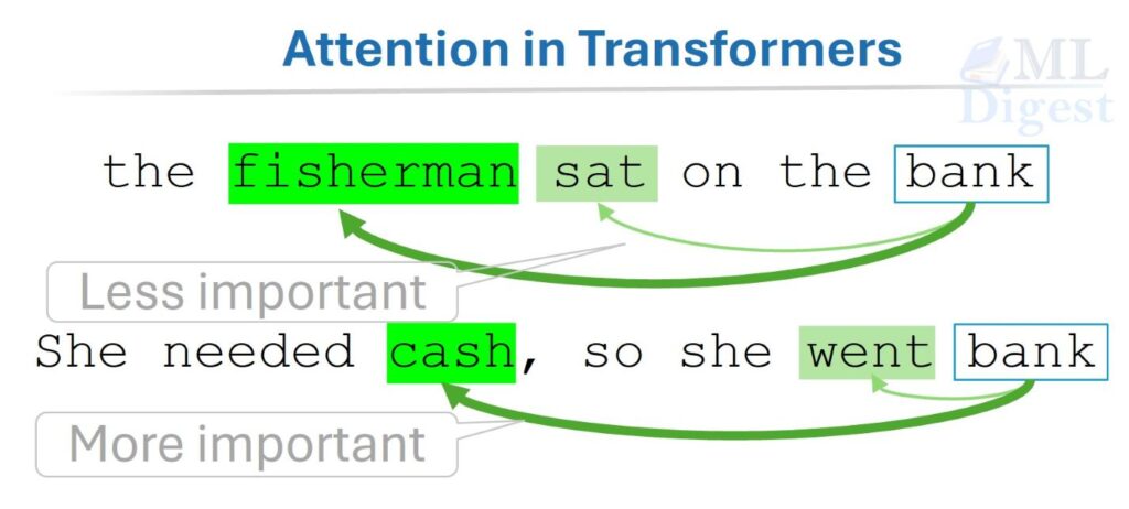
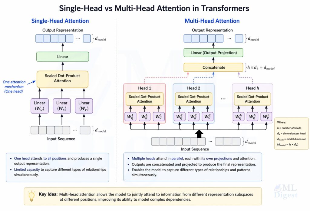
4.3 Masked Multi-Head Self-Attention
Self-attention is the mechanism that allows each token to “look at” other tokens in the sequence and gather context. For a fuller conceptual treatment, see attention mechanism in transformers. For a single attention head, given an input matrix $H \in \mathbb{R}^{T \times d}$:
$$Q = H W_Q, \quad K = H W_K, \quad V = H W_V$$
where $W_Q, W_K, W_V \in \mathbb{R}^{d \times d_k}$ are learned projection matrices. The attention output is:
$$\text{Attention}(Q, K, V) = \text{softmax}\left(\frac{QK^\top}{\sqrt{d_k}} + M\right) V$$
The matrix $M$ is the causal mask: it sets entries to $-\infty$ wherever position $j > i$, so that position $i$ can only attend to positions $1$ through $i$. After the softmax, these entries become zero, meaning no information from future tokens leaks into the current prediction.
Multi-head attention runs $h$ such attention heads in parallel, each with its own projection matrices, and concatenates the results:
$$\text{MHA}(H) = \text{Concat}(\text{head}_1, \ldots, \text{head}_h) W_O$$
where $W_O \in \mathbb{R}^{hd_k \times d}$ is another learned projection. This allows the model to capture different types of relationships between tokens in different subspaces.
4.4 Feed-Forward Network
After attention, each token’s representation passes through a two-layer feed-forward network applied independently at each position:
$$\text{FFN}(x) = \text{GELU}(x W_1 + b_1) W_2 + b_2$$
where $W_1 \in \mathbb{R}^{d \times 4d}$ and $W_2 \in \mathbb{R}^{4d \times d}$. The inner dimension is typically four times the model dimension. GPT uses the GELU activation function rather than ReLU, which tends to give smoother gradients in practice.
4.5 Residual Connections and Layer Normalization
Each sub-layer is wrapped in a residual connection and a layer normalization. Modern implementations of GPT use the “pre-norm” formulation, where layer normalization is applied before the sub-layer:
$$x \leftarrow x + \text{Sublayer}(\text{LayerNorm}(x))$$
The residual connections enable gradients to flow directly to earlier layers during backpropagation, which is critical when stacking dozens or hundreds of layers. Layer normalization stabilizes the activation magnitudes across the sequence dimension, making training more reliable.
In original Transformer implementations, “post-norm” was used (layer normalization after the sub-layer), but pre-norm has become more common in GPT models due to improved training stability, especially at larger scales. Post-norm formulation is given by:
$$x \leftarrow \text{LayerNorm}(x + \text{Sublayer}(x))$$
In practice, pre-norm became standard in GPT-style models because it scales more reliably to deeper stacks.
4.6 Training Versus Inference
One subtle but important point is that GPT is trained and used in slightly different ways.
During training, the full token sequence is available, and the model predicts every next-token target in parallel under the causal mask. During inference, generation is sequential: the model predicts one new token, appends it to the context, and runs again. The architecture is the same in both cases, but inference is inherently slower because it unfolds one step at a time.
5. Pre-Training, Instruction Tuning, and Alignment
5.1 Pre-Training
During pre-training, GPT processes token sequences from a large corpus and minimizes cross-entropy loss against the true next token. For a sequence of length $T$:
$$\mathcal{L}_{\text{pre}} = -\frac{1}{T}\sum_{t=1}^{T} \log P_\theta(x_t \mid x_{<t})$$
Optimization is typically performed with adaptive gradient methods such as Adam or AdamW over many millions of sequences on distributed GPU clusters. This is the expensive stage that gives the model its broad language competence.
5.2 Supervised Fine-Tuning and Preference Alignment
Raw next-token prediction is not enough to produce a helpful assistant. After pre-training, models are often adapted with supervised fine-tuning (SFT) on high-quality prompt-response pairs.
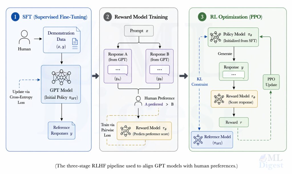
For instruction-following systems such as ChatGPT, post-training typically combines SFT with human-preference-based alignment methods. Historically this has included Reinforcement Learning from Human Feedback (RLHF), while newer systems may also use other preference-optimization methods. The core idea is to incorporate human judgments into training so that model outputs become more useful, safer, and better aligned with user intent.
The original InstructGPT pipeline proceeds in three stages:
- SFT: Fine-tune the pre-trained model on demonstrations written by human annotators.
- Reward modeling: Collect human preference comparisons between candidate outputs and train a separate model to score them.
- Policy optimization: Use Proximal Policy Optimization (PPO) to improve the language model against the learned reward while constraining it not to drift too far from the supervised policy.
The important conceptual point is that pre-training teaches broad competence, while alignment and fine-tuning shape how that competence is expressed.
6. The GPT Family: What Changed Across Generations
Each generation of GPT retained the decoder-only foundation, but scale, data, optimization, and alignment methods improved dramatically.
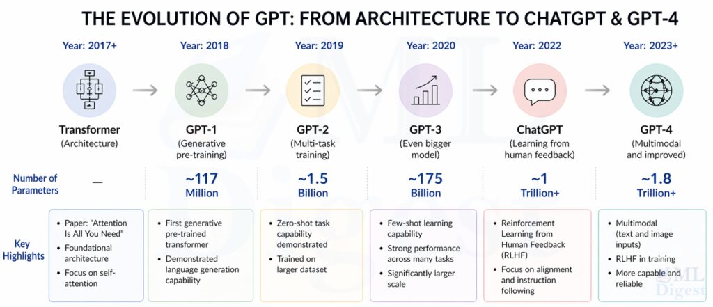
6.1 GPT-1 (2018)
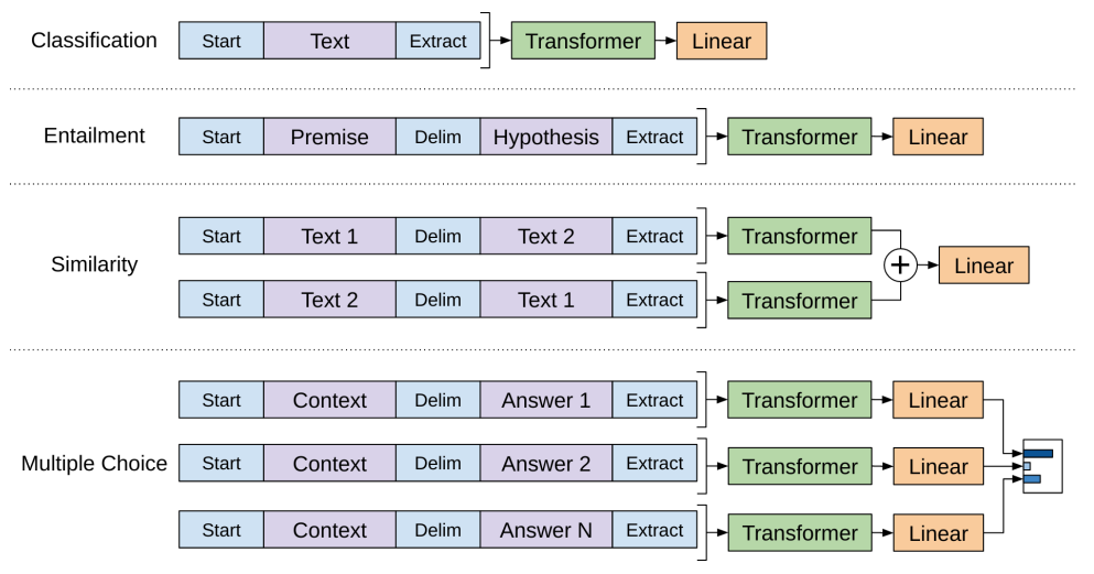
GPT-1 (Radford et al., 2018) had 117 million parameters, with 12 layers, 12 attention heads, and hidden size 768. It was trained on BooksCorpus, a dataset of more than 7,000 unpublished books. Its key result was strategic rather than purely benchmark-based: a single generative pre-trained model could be fine-tuned effectively across many NLP tasks.
6.2 GPT-2 (2019)
GPT-2 (Radford et al., 2019) scaled to 1.5 billion parameters and was trained on WebText. It showed that sufficiently large language models can perform translation, summarization, and question answering in a zero-shot or prompt-based way, without task-specific gradient updates. OpenAI initially staged the release because the generated text was considered realistic enough to pose misuse risks.
6.3 GPT-3 (2020)
GPT-3 (Brown et al., 2020) expanded to 175 billion parameters and used a 2,048-token context window. It was trained on a mixture that included Common Crawl, WebText, books, and Wikipedia. GPT-3 made in-context learning a central practical idea: with zero-shot, one-shot, or few-shot prompting, the same model could perform many tasks it was never explicitly fine-tuned for.
6.4 InstructGPT and GPT-3.5 (2022)
InstructGPT showed that a smaller but aligned model can be substantially more useful than a larger raw next-token predictor. The label GPT-3.5 is best understood as a family of models in the transition between GPT-3 and GPT-4, with stronger instruction-following and dialogue behavior produced through supervised tuning and human preference optimization.
6.5 GPT-4 (2023)
The GPT-4 technical report describes GPT-4 (OpenAI, 2023) as a large-scale multimodal model that can accept image and text inputs and produce text outputs. Public details about architecture and parameter count remain limited, so discussions of GPT-4 are necessarily less concrete than discussions of GPT-1 through GPT-3. Even with that limitation, the report and subsequent deployments indicate improved performance on many reasoning, factuality, and instruction-following evaluations.
7. Building Intuition with Code
The concepts above are easiest to internalize when you see them in a compact implementation. The following PyTorch example keeps the architecture minimal while preserving the essential GPT ingredients: token embeddings, positional embeddings, masked self-attention, feed-forward blocks, residual paths, and a tied output head.
import math
import torch
import torch.nn as nn
import torch.nn.functional as F

class CausalSelfAttention(nn.Module):
    """Multi-head masked self-attention."""

    def __init__(self, d_model: int, n_heads: int, seq_len: int, dropout: float = 0.1):
        super().__init__()
        assert d_model % n_heads == 0
        self.n_heads = n_heads
        self.d_k = d_model // n_heads

        # Single projection for Q, K, V to keep things efficient
        self.qkv_proj = nn.Linear(d_model, 3 * d_model, bias=False)
        self.out_proj = nn.Linear(d_model, d_model, bias=False)
        self.attn_dropout = nn.Dropout(dropout)

        # Causal mask: upper triangle is -inf so future tokens are invisible
        mask = torch.triu(torch.ones(seq_len, seq_len), diagonal=1).bool()
        self.register_buffer("mask", mask)

    def forward(self, x: torch.Tensor) -> torch.Tensor:
        B, T, C = x.shape  # batch, sequence length, model dimension

        # Compute Q, K, V in one matmul and split
        q, k, v = self.qkv_proj(x).split(C, dim=-1)

        # Reshape to (B, n_heads, T, d_k) for batched attention
        def reshape(t):
            return t.view(B, T, self.n_heads, self.d_k).transpose(1, 2)

        q, k, v = reshape(q), reshape(k), reshape(v)

        # Scaled dot-product attention with causal mask
        scores = (q @ k.transpose(-2, -1)) / math.sqrt(self.d_k)
        scores = scores.masked_fill(self.mask[:T, :T], float("-inf"))
        weights = self.attn_dropout(F.softmax(scores, dim=-1))

        # Weighted sum of values, then merge heads
        out = (weights @ v).transpose(1, 2).contiguous().view(B, T, C)
        return self.out_proj(out)


class TransformerBlock(nn.Module):
    """A single GPT decoder block: attention -> FFN, each with residual + LayerNorm."""

    def __init__(self, d_model: int, n_heads: int, seq_len: int, dropout: float = 0.1):
        super().__init__()
        self.ln1 = nn.LayerNorm(d_model)
        self.attn = CausalSelfAttention(d_model, n_heads, seq_len, dropout)
        self.ln2 = nn.LayerNorm(d_model)
        self.ffn = nn.Sequential(
            nn.Linear(d_model, 4 * d_model),
            nn.GELU(),
            nn.Linear(4 * d_model, d_model),
            nn.Dropout(dropout),
        )

    def forward(self, x: torch.Tensor) -> torch.Tensor:
        # Pre-norm formulation (used in practice for stability)
        x = x + self.attn(self.ln1(x))
        x = x + self.ffn(self.ln2(x))
        return x


class GPT(nn.Module):
    """Minimal decoder-only GPT model."""

    def __init__(
        self,
        vocab_size: int,
        seq_len: int,
        d_model: int,
        n_layers: int,
        n_heads: int,
        dropout: float = 0.1,
    ):
        super().__init__()
        self.token_emb = nn.Embedding(vocab_size, d_model)
        self.pos_emb = nn.Embedding(seq_len, d_model)
        self.drop = nn.Dropout(dropout)
        self.blocks = nn.Sequential(
            *[TransformerBlock(d_model, n_heads, seq_len, dropout) for _ in range(n_layers)]
        )
        self.ln_final = nn.LayerNorm(d_model)
        # Weight tying: share weights between token embedding and output projection
        # (reduces parameters and improves generalization)
        self.head = nn.Linear(d_model, vocab_size, bias=False)
        self.head.weight = self.token_emb.weight

    def forward(self, idx: torch.Tensor) -> torch.Tensor:
        B, T = idx.shape
        positions = torch.arange(T, device=idx.device)

        # Token embeddings + positional embeddings
        x = self.drop(self.token_emb(idx) + self.pos_emb(positions))

        # Pass through all transformer blocks
        x = self.blocks(x)
        x = self.ln_final(x)

        # Project to vocabulary logits
        return self.head(x)  # shape: (B, T, vocab_size)


# --- Smoke test ---
if __name__ == "__main__":
    model = GPT(vocab_size=50257, seq_len=1024, d_model=768, n_layers=12, n_heads=12)
    total_params = sum(p.numel() for p in model.parameters())
    print(f"Parameters: {total_params / 1e6:.1f}M")  # ~124M (weights are tied)

    dummy_input = torch.randint(0, 50257, (2, 16))  # batch of 2, length 16
    logits = model(dummy_input)
print(f"Output shape: {logits.shape}") # (2, 16, 50257)A few implementation details are worth noticing:
- Weight tying: The token embedding matrix and the final output projection share weights, a technique introduced by Press and Wolf (2016). This reduces parameters and often improves language modeling quality.
- Pre-norm formulation: Layer normalization is applied before each sub-layer. This is one reason modern GPT stacks train more stably than a direct post-norm implementation.
- Causal mask as a buffer: The mask is stored as a non-parameter buffer so it moves with the model across devices automatically.
7.1 Autoregressive Text Generation
Once the model is trained, generation is conceptually simple: run the model on the current context, sample the next token from the output distribution, append it, and repeat.
@torch.no_grad()
def generate(
    model: GPT,
    idx: torch.Tensor,
    max_new_tokens: int,
    temperature: float = 1.0,
    top_k: int = None,
) -> torch.Tensor:
    """
    Autoregressively generate tokens from a prompt.

    Args:
        model:          Trained GPT model.
        idx:            (1, T) integer tensor of prompt token ids.
        max_new_tokens: Number of tokens to generate.
        temperature:    Scales logits before softmax. Lower = more focused.
        top_k:          If set, only sample from the top-k most likely tokens.
    """
    model.eval()
    seq_len = model.pos_emb.num_embeddings  # maximum context length

    for _ in range(max_new_tokens):
        # Truncate to the model's context window if necessary
        idx_cond = idx[:, -seq_len:]

        # Forward pass to get logits for the last position
        logits = model(idx_cond)[:, -1, :]  # (1, vocab_size)

        # Apply temperature scaling
        logits = logits / temperature

        # Optionally restrict to top-k candidates
        if top_k is not None:
            values, _ = torch.topk(logits, top_k)
            logits[logits < values[:, -1:]] = float("-inf")

        # Sample from the distribution
        probs = F.softmax(logits, dim=-1)
        next_token = torch.multinomial(probs, num_samples=1)

        # Append the new token and continue
        idx = torch.cat([idx, next_token], dim=1)

return idxThe temperature parameter controls how concentrated the sampling distribution is. A lower temperature, such as 0.7, makes the model more conservative. A higher temperature increases diversity, but also raises the chance of incoherent completions. The top_k filter adds another practical control by limiting sampling to the most likely candidates. In production systems, repeated decoding is usually accelerated with a KV cache, which avoids recomputing every past key and value tensor from scratch at each step.
8. Why GPT Became So Useful
GPT models became broadly useful because they combine a small number of powerful ideas:
- A universal objective: next-token prediction applies to almost any text corpus.
- Global context mixing: self-attention allows every token to integrate information from the full visible context.
- Transfer through pre-training: one large model can serve many downstream tasks.
- Prompt-based adaptation: later GPT models often need only instructions or examples, not task-specific retraining.
- Predictable gains from scale: scaling laws show that performance often improves smoothly with more data, parameters, and compute.
These properties explain the range of applications now associated with GPT systems: conversational assistants, coding tools such as GitHub Copilot, drafting and editing support, question answering over documents, summarization, tutoring, and workflow automation.
9. Limitations and Risks
Despite their fluency, GPT models have important limitations.
- Hallucination: A GPT model can generate text that is plausible and polished but factually wrong. The training objective rewards likely continuations, not verified truth.
- No genuine understanding: GPT operates on statistical patterns in text. It does not have a grounded model of the world, sensory experience, or human values.
- Bias inheritance: Because training data reflects human society, the model can reproduce harmful stereotypes and uneven representation.
- High compute cost: Training and serving large models requires substantial infrastructure, energy, and optimization effort.
- Context limitations: Long context windows help, but they do not fully solve retrieval, long-horizon consistency, or attention dilution in very large documents.
- Prompt sensitivity: Small changes in wording, examples, or formatting can materially change output quality.
There are also broader societal concerns:
- Misinformation and synthetic media: High-quality generated text lowers the cost of spam, propaganda, and manipulation.
- Academic and professional misuse: Text generation can be used to misrepresent authorship or expertise.
- Labor disruption: Writing, support, and analysis workflows are increasingly automated, which creates both productivity gains and displacement pressure.
- Alignment remains incomplete: Methods such as SFT and RLHF improve behavior, but they do not eliminate failure modes or guarantee robust safety.
Closing Thoughts
GPT’s progression from a 117-million-parameter proof of concept in 2018 to a multimodal system capable of passing professional exams in 2023 is one of the most consequential arcs in modern machine learning.
GPT is one of the clearest examples in modern machine learning of a simple objective producing unexpectedly broad capability. Predicting the next token does not sound like a general intelligence recipe, yet when combined with Transformer decoders, large-scale data, and enough compute, it yields systems that can write, summarize, translate, explain, and assist across a striking range of domains.
The important lesson is not that GPT is magic. It is that architecture, objective, scale, and alignment interact in a very particular way. Once those pieces are clear, GPT becomes much less mysterious and much easier to evaluate critically.
References
- Vaswani, A., et al. (2017). Attention Is All You Need. NeurIPS.
- Sennrich, R., Haddow, B., and Birch, A. (2016). Neural Machine Translation of Rare Words with Subword Units. ACL.
- Radford, A., et al. (2018). Improving Language Understanding by Generative Pre-Training. OpenAI.
- Radford, A., et al. (2019). Language Models are Unsupervised Multitask Learners. OpenAI.
- Devlin, J., et al. (2018). BERT: Pre-training of Deep Bidirectional Transformers for Language Understanding.
- Brown, T., et al. (2020). Language Models are Few-Shot Learners. NeurIPS.
- Kaplan, J., et al. (2020). Scaling Laws for Neural Language Models. OpenAI.
- Ouyang, L., et al. (2022). Training language models to follow instructions with human feedback. NeurIPS.
- OpenAI. (2023). GPT-4 Technical Report.
- Press, O., and Wolf, L. (2016). Using the Output Embedding to Improve Language Models.
- Hendrycks, D., and Gimpel, K. (2016). Gaussian Error Linear Units (GELUs).
- Christiano, P., et al. (2017). Deep Reinforcement Learning from Human Preferences. NeurIPS.
- Schulman, J., et al. (2017). Proximal Policy Optimization Algorithms.

Happy is a seasoned ML professional with over 15 years of experience. His expertise spans various domains, including Computer Vision, Natural Language Processing (NLP), and Time Series analysis. He holds a PhD in Machine Learning from IIT Kharagpur and has furthered his research with postdoctoral experience at INRIA-Sophia Antipolis, France. Happy has a proven track record of delivering impactful ML solutions to clients.

Silpa brings 5 years of experience in working on diverse ML projects, specializing in designing end-to-end ML systems tailored for real-time applications. Her background in statistics (Bachelor of Technology) provides a strong foundation for her work in the field. Silpa is also the driving force behind the development of the content you find on this site.
Subscribe to our newsletter!