Approximate nearest neighbor (ANN) search is a family of algorithms and systems for quickly answering a deceptively simple question:
Given a query vector, which database vectors are most similar to it?
This question appears throughout modern ML pipelines: semantic search, retrieval-augmented generation (RAG), recommendation systems, entity resolution, anomaly detection, and near-duplicate detection. At millions or billions of vectors, scoring every candidate exactly is often too slow or too costly.
ANN deliberately trades a controlled amount of retrieval quality for much lower latency, higher throughput, and, in some methods, lower memory use. The goal is not merely to search faster, but to meet a quality target within a fixed systems budget.
1. The Core Idea (Intuition)
Imagine a library with millions of books. Given a query, you want the $k$ most similar books.
- Exact nearest neighbors read every summary and rank every book. They provide the reference answer, but require work proportional to the full collection.
- Approximate nearest neighbors use a catalog that first identifies promising shelves, then inspect only a small candidate set. The returned items may not be the exact top $k$, but they are often sufficient for the downstream task.
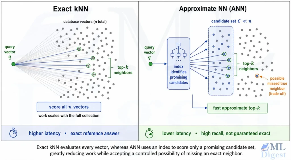
That catalog can take several forms:
- Hashing: put similar vectors into the same buckets (probabilistically).
- Trees: partition space and skip large irrelevant regions.
- Quantization: compress vectors so distance computations become cheaper.
- Graphs: build a navigable network of neighbors and walk it efficiently.
The vectors being compared are usually produced by an embedding model that maps raw items, such as text, images, or users, into points in $\mathbb{R}^d$; see text embeddings for how that mapping is learned for language.
2. Why ANN Matters in Practice
ANN becomes important when exact $k$-nearest-neighbor (kNN) search is the bottleneck, particularly when the collection is large and latency requirements are strict.
2.1 Common use cases
- Semantic search: retrieve the most relevant documents for a query embedding.
- Recommendations: retrieve similar user or item embeddings; for example how the Twitter/X recommendation engine works for a large-scale production example.
- RAG retrieval: retrieve passages to condition a language model. The passages an ANN index can retrieve are only as good as how the source documents were split beforehand, so chunking strategy is a direct input to retrieval quality.
- Hybrid retrieval: combine ANN semantic search with a lexical ranker such as BM25 when exact terms, identifiers, or rare phrases must remain retrievable.
- Deduplication: find near-duplicates in images/text/audio.
- Entity resolution: find candidate matches before running a slower matching model.
2.2 What you usually optimize
In a production system, the best index is a multi-objective choice:
- Quality: Recall@k (or Recall@R where $R$ is the retrieval depth), NDCG, or task-level metrics.
- Latency: p50/p95/p99 query time.
- Throughput: queries per second (QPS).
- Memory: index size plus stored vectors.
- Build time: how long it takes to construct (or rebuild) an index.
- Update support: ability to add and delete vectors online, versus periodic rebuilds.
ANN exposes parameters that let you tune these objectives against one another.
3. Formal Problem Statement and Key Math
Let $\mathcal{X} = {x_1, x_2, \dots, x_n}$ be a set of vectors $x_i \in \mathbb{R}^d$ and let $q \in \mathbb{R}^d$ be a query vector.
For a distance metric $\delta$, the exact $k$-nearest-neighbor problem returns:
$$
\operatorname{kNN}_k(q; \mathcal{X}) = \underset{\substack{I \subseteq {1,\ldots,n}\ |I|=k}}{\operatorname{arg\,min}} \;\sum_{i \in I} \delta(q, x_i).
$$
ANN returns an approximation to these neighbors, typically by searching a subset of candidates. A system may approximate the neighbor set, the scores, or both.
3.1 Distances and similarities you actually use
In embedding retrieval, these are the usual choices:
- Euclidean (L2) distance
$$d_2(q, x) = \lVert q – x \rVert_2$$ - Inner product (dot product)
$$s(q, x) = q^\top x$$
If you treat this as a “distance,” you usually want maximum inner product. - Cosine similarity
$$\cos(q, x) = \frac{q^\top x}{\lVert q \rVert_2 \lVert x \rVert_2}$$
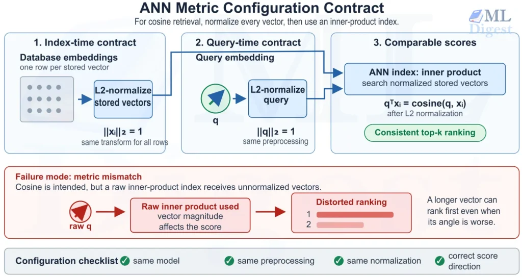
If both vectors are L2-normalized, cosine similarity and inner product produce the same ranking. This equivalence makes metric handling a critical index configuration decision.
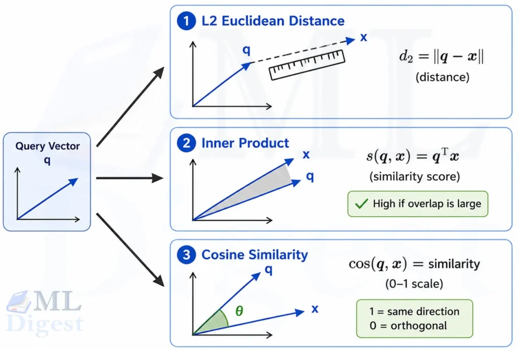
Distance and similarity functions can rank the same vectors differently. Use the metric that matches the embedding model and configure the index consistently.
3.2 Why brute force is slow
Exact search compares $q$ to all $n$ vectors:
- Dense scoring costs $\mathcal{O}(nd)$ per query, before selecting the top $k$ results.
- Fast matrix kernels and GPUs can make brute-force search practical at moderate scale, but they cannot remove the need to read and score every vector.
ANN aims to reduce the number of full distance computations from $n$ to something closer to a small candidate set $C \ll n$.
3.3 A common approximation definition (useful vocabulary)
Many papers formalize ANN using a $(c, r)$-approximate nearest-neighbor definition:
- $r > 0$ is a distance threshold. Suppose there exists at least one database point $x \in \mathcal{X}$ such that $\delta(q, x) \le r$.
- $c \ge 1$ is the approximation factor. An algorithm is $(c, r)$-approximate if it returns a point $\hat{x}$ satisfying
$$
\delta(q, \hat{x}) \le c r.
$$ - A smaller $c$ is a stronger guarantee: when the premise holds, $c=1$ requires the algorithm to return a point within $r$, while larger values allow the returned point to be farther away.
Production systems rarely enforce this strict guarantee. They usually optimize empirical metrics such as Recall@k under a latency budget. The definition remains useful when reading ANN research.
4. What Makes Nearest Neighbor Search Hard
Two practical realities shape ANN design:
- The curse of dimensionality: many classic spatial data structures degrade as $d$ grows. Intuitively, high-dimensional space is “sparse,” and distances can become less informative.
- Real embeddings are not uniform random points: they are often clustered, anisotropic, and model-dependent. ANN methods that exploit this structure (especially graph-based methods) often perform very well.
5. Main ANN Families
The following families use different shortcuts. Understanding the shortcut is more useful than memorizing a library-specific index name.
5.1 Tree-based methods (KD-tree, Ball tree)
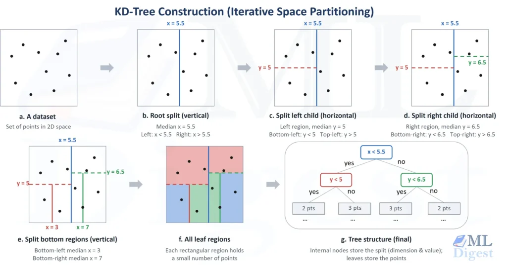
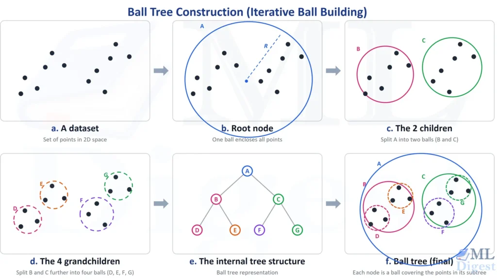
Partition the space recursively into rectangles for a K-dimensional tree (KD-tree) or hyperspheres for a Ball tree. During a query, the index prunes regions that cannot contain a closer neighbor.
Key idea: skip large regions that cannot contain a close neighbor.
How the index is built and queried:
- Build a KD-tree: choose a split dimension, commonly the dimension with the largest spread, split the points near the median on that coordinate, and recurse until each leaf contains only a small number of points. Each internal node represents an axis-aligned rectangular region.
- Build a Ball tree: group nearby points into a hypersphere with center $c$ and radius $R$, split the group into two compact child groups, compute a bounding sphere for each child, and recurse to small leaves. This structure can adapt better than axis-aligned rectangles when clusters are not aligned with the coordinate axes.
- Search the promising child first: descend to the child whose rectangle or sphere is closer to the query, while maintaining the best $k$ points found so far in a bounded priority queue.
- Prune safely: skip a KD-tree region when its minimum possible distance to the query exceeds the current worst retained neighbor. For a Ball-tree node, a lower bound is $\max(0, \delta(q,c)-R)$; skip the node when this bound is already too large.
- Make search approximate when needed: cap the number of visited nodes or leaves, or stop backtracking early. This reduces latency but can miss an exact neighbor.
When to consider them:
- Often strong for low-to-moderate dimensions.
- Typically degrade as dimension increases, although the data distribution matters.
- Useful as an interpretable baseline and widely available in general-purpose libraries.
5.2 Hashing and locality-sensitive hashing (LSH)
LSH uses a randomized hash family whose collision probability is higher for nearby vectors than for distant ones. A query searches only vectors in its matching hash buckets, then scores those candidates with the target similarity or distance function.
Key idea: make collision probability correlate with similarity.
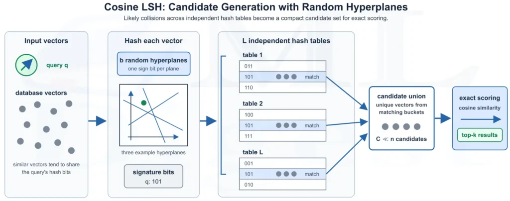
For cosine similarity, a standard LSH family uses random hyperplanes. Given a random vector $r$ drawn from a spherically symmetric distribution, define
$$
h_r(x) = \operatorname{sign}(r^\top x).
$$
The hyperplane perpendicular to $r$ divides the space into two half-spaces. Two vectors on the same side of the hyperplane receive the same bit.
Thus, vectors with a small angle, and therefore high cosine similarity, collide more often. More precisely, two vectors at angle $\theta$ collide with probability $1 – \frac{\theta}{\pi}$. A practical index combines several such bits into a signature and uses multiple hash tables:
- Sample $b$ random hyperplanes and concatenate their output bits into one $b$-bit signature. Each signature selects a bucket in one table.
- $L$ is the number of independently randomized hash tables. Each table uses its own $b$ random hyperplanes, so every database vector is stored once per table, potentially in a different bucket each time.
- At query time, look up the query’s bucket in all $L$ tables and take the union of their vectors. A true neighbor needs to collide with the query in only one table to become a candidate, which raises recall; nearby buckets can also be probed when needed.
- Score the resulting candidates with cosine similarity or another intended metric, then return the top $k$.
More bits $b$ make individual buckets smaller and reduce unnecessary candidates, but can also separate true neighbors. More tables $L$, or additional bucket probes, increases the chance of finding true neighbors at the cost of memory and query work.
Pros:
- Provides probabilistic similarity guarantees for a specified hash family.
- Bucket construction and lookup are simple and can be parallelized or distributed.
Cons:
- High recall can require many tables, bucket probes, or candidates, increasing memory and query cost.
- On many modern dense-embedding workloads, graph-based indexes achieve better recall-latency trade-offs.
5.3 Quantization and inverted indexes (IVF, PQ, IVF-PQ)
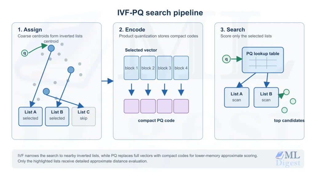
An inverted file (IVF) assigns each vector to a coarse centroid and stores it in that centroid’s list. A query visits only its best-matching lists under the configured metric. Product quantization (PQ) then compresses vectors as short code sequences, allowing many approximate distance or similarity calculations to be implemented as table lookups.
IVF and PQ are complementary, not competing approaches. IVF decides where to search, reducing the number of candidate vectors. PQ decides how vectors are stored and scored, reducing memory use and the cost of comparing each candidate. They can be used separately, but IVF-PQ combines both benefits.
Inverted file (IVF), a candidate-selection method
- Train a coarse quantizer with $n_{\mathrm{list}}$ centroids, for example with k-means.
- Assign each database vector to its best-matching centroid under the index metric (the nearest centroid for L2 distance) and store it in that centroid’s inverted list.
- At query time, score the coarse centroids and search only the best-matching $n_{\text{probe}}$ lists.
- IVF can be used without PQ: an IVF-Flat index keeps full-precision vectors in each selected list and scores them exactly.
Product quantization (PQ), a compression and approximate-scoring method
- Split each $d$-dimensional vector into $m$ sub-vectors and train a small codebook for each subspace.
- Replace every sub-vector with the ID of its nearest codeword. For example, 256 codewords require 8 bits per sub-vector.
- At query time, precompute a small lookup table of query-to-codeword values, then combine its entries to estimate each vector’s distance or similarity.
- PQ can be used without IVF, but then the system typically scans compressed codes from the entire collection or uses another candidate-selection method.
For IVF-PQ, the usual order is:
- Build: train the IVF coarse quantizer, then train PQ codebooks on representative vectors, often on residuals relative to the assigned coarse centroids. Assign each database vector to an inverted list and encode its vector or residual $x-c_j$ using the trained PQ codebooks.
- Query: choose the best-matching $n_{\mathrm{probe}}$ IVF lists first, then use metric-specific PQ lookup values to score only the compressed codes in those lists.
- Optional reranking: retain full vectors for the strongest candidates and rescore them exactly before returning the final top $k$.
Thus, IVF reduces the search space first, while PQ makes the remaining comparisons compact and fast. The combined approach trades some recall for lower memory use and lower query cost.
Where it shines:
- Very large collections, especially when storing full-precision vectors is expensive.
- When memory is a constraint.
- When you can accept some quantization error.
Graph-based ANN is a frequent default for embedding retrieval because it often delivers excellent recall within a low-latency budget.
Each vector is a node linked to a small set of neighbors. Search begins from an entry point and repeatedly moves toward closer nodes. In HNSW, sparse upper layers make large jumps across the graph before a dense lower layer refines the candidate set.
One widely used graph index is HNSW (Hierarchical Navigable Small World).
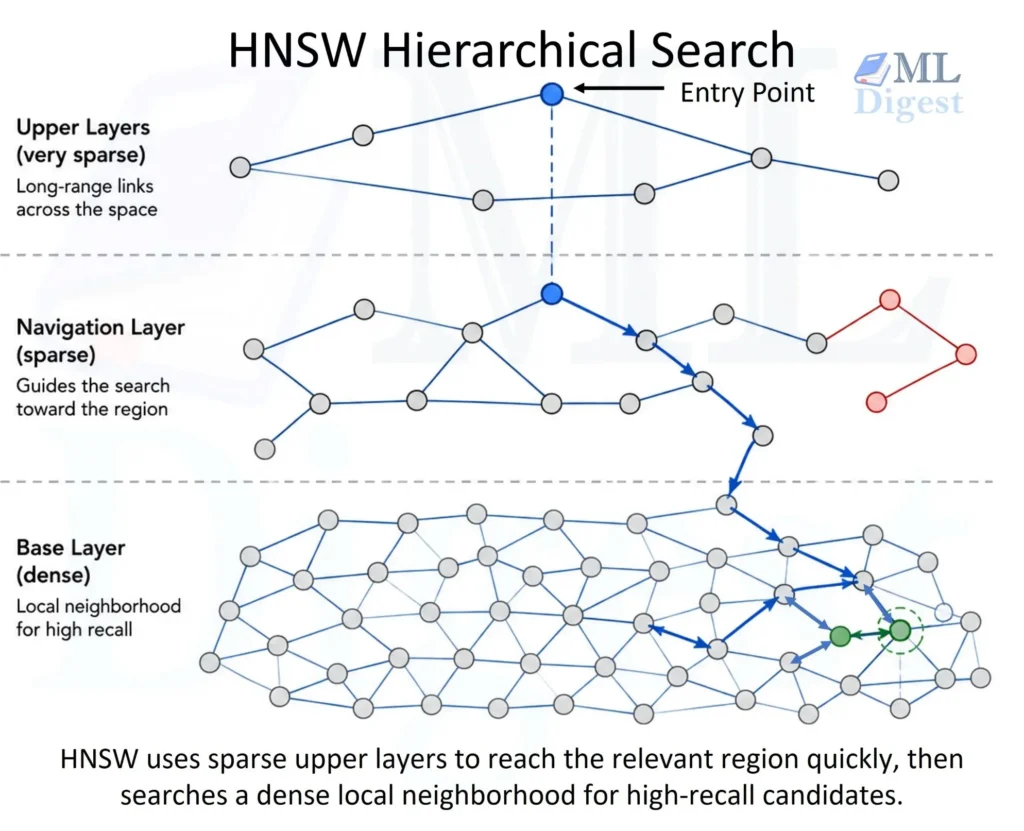
- Index build: insert points one at a time and link each point to selected neighbors, subject to a degree limit.
- Multiple layers: upper layers are sparse express lanes that quickly reach the right region; the lowest layer performs the detailed search.
- Search: use greedy traversal at upper layers and a broader best-first search at the bottom layer.
6. How to Choose an ANN Method
There is no universally best ANN index. The choice depends on collection size, vector dimension, similarity metric, hardware, memory budget, filtering requirements, and update pattern.
6.1 Quick decision guidelines
- For high-dimensional embeddings with a high-recall requirement and sufficient memory, begin with HNSW.
- For very large collections or tight memory budgets, evaluate IVF-PQ, often with reranking against full vectors for the retained candidates.
- For workloads that value theoretical collision guarantees or simple distributed hashing, consider LSH.
- For low-dimensional, well-behaved data, a KD-tree or Ball tree may be sufficient.
6.2 Important system constraints
- Updates: many indices support incremental inserts, but deletion support and its cost vary by index. Frequent deletes or massive churn can degrade performance or require compaction and rebuilds.
- Filters: if you need metadata filtering (for example, language, tenant, category), the index strategy changes.
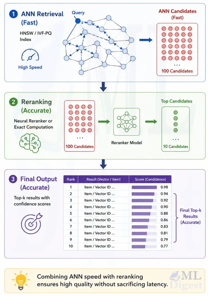
- Reranking: if the service can retrieve $R$ candidates quickly and rerank them with exact scoring or a stronger model, the ANN stage can prioritize recall over precision at $k$. This mirrors the two-stage reranking pattern used in RAG pipelines, where a cheap retriever’s candidates are re-scored by a more precise model before the final context is assembled. A common neural design uses a fast bi-encoder retriever followed by a more expensive cross-encoder reranker.
6.3 How to evaluate an ANN index
ANN quality is not a single number. Evaluate candidate indexes with a query set that represents production traffic, measuring quality alongside latency, memory, and operational costs.
- Recall@k (most common):
- On the same representative database subset used for ANN evaluation, compute the exact and approximate top-$k$ neighbors, then measure their overlap.
- $$\text{Recall@k} = \frac{|\text{ANN@k}(q) \cap \text{Exact@k}(q)|}{k}$$
- Report the average across all evaluation queries, together with dispersion or a low percentile when query difficulty varies substantially.
- This retrieval Recall@k borrows its name from the classic precision and recall metric family, but it measures candidate-set overlap rather than true/false positive rates.
- Recall@N for “retrieve $N$ then rerank”:
- In many stacks, ANN retrieves $N$ candidates, then a second-stage model reranks.
- In this case, Recall@$N$ is often more important than Recall@k.
- Latency percentiles: p50, p95, and p99, measured under a representative concurrency level.
- Build time and index size: include the cost of retraining, loading, and serving replicas where relevant.
When ANN supplies RAG context, pair these retrieval metrics with end-to-end RAG evaluation so the chosen operating point also supports answer quality.
7. Implementation Steps (End-to-End)
The following sequence creates a measurable baseline before committing to a production index.
7.1 Step 1: Define your retrieval objective
- What is the downstream task: search, recommendation, or candidate generation?
- Which metric aligns with success: task-level AUC, CTR, NDCG, or MRR?
- What is the p95 or p99 latency budget, including all downstream stages?
7.2 Step 2: Choose a distance metric and normalize consistently
Common pattern for embeddings:
- For cosine similarity, L2-normalize vectors at both indexing and query time.
- Use
float32unless measurement justifies another representation.
7.3 Step 3: Build an exact baseline on a sample
Before doing ANN, establish reference numbers:
- Select a representative database subset, for example 50,000 to 500,000 vectors, and run exact kNN over that same subset for every evaluation query.
- Measure exact latency and memory in the same environment that will host ANN experiments.
- Use the exact results as ground truth for Recall@k and Recall@$R$.
- Keep the corpus and embedding snapshot fixed while generating exact and ANN results; point-in-time correctness prevents data changes from contaminating recall measurements.
7.4 Step 4: Pick an ANN library and index type
Common Python-accessible options include:
hnswlib: a lightweight HNSW implementation.- FAISS: a broad CPU and GPU toolkit with IVF, PQ, HNSW, and more.
- Annoy: a simple tree-based option for suitable workloads.
See tools and frameworks for machine learning for how these libraries fit into the broader ML tooling landscape.
Library choice does not replace evaluation. Compare candidate indexes on your data, metric, filter behavior, and target hardware.
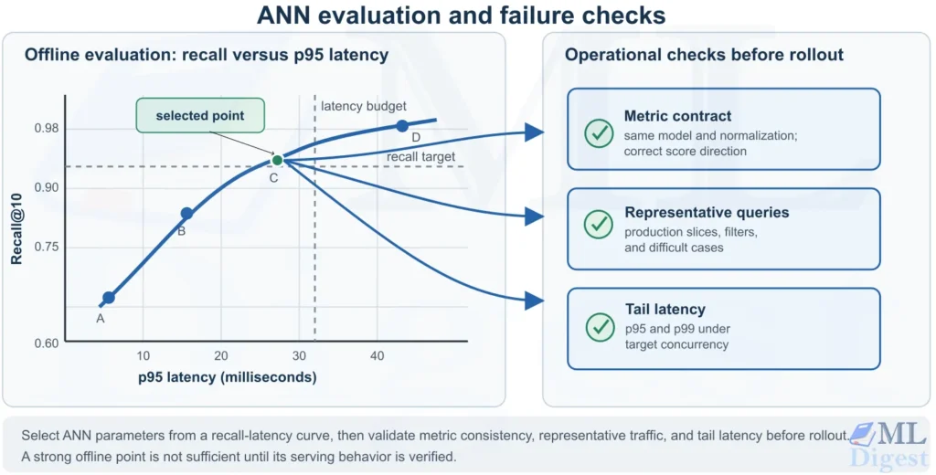
7.5 Step 5: Tune ANN parameters using a recall–latency curve
Produce a parameter sweep rather than choosing settings by intuition:
- Fix a dataset sample and a query set.
- Sweep
efSearch,M,nprobe, etc. - Plot (or tabulate) Recall@k versus p95 latency.
Choose a point near the knee of the curve, where additional latency yields only small quality gains.
7.6 Step 6: Add a reranking stage (optional but common)
If you store full vectors, a strong pattern is:
- ANN retrieves top $R$ candidates quickly.
- Compute exact distances or a learned scoring model on those $R$.
- Return top $k$.
This often produces near-exact final quality while preserving ANN-scale retrieval latency.
7.7 Step 7: Deploy with monitoring and guardrails
In production, measure continuously:
- latency (p50/p95/p99)
- queries per second (QPS)
- retrieval-quality proxy metrics, for example overlap with a slower exact service on a sampled query stream
- index health (size, build time, update lag)
Instrument these signals with a standard observability stack such as OpenTelemetry so ANN latency and throughput stay comparable with the rest of the serving pipeline.
7.8 Step 8: Engineer for scale (shards, batching, persistence)
After establishing a good recall-latency configuration on one machine, further progress is often a systems-design problem.
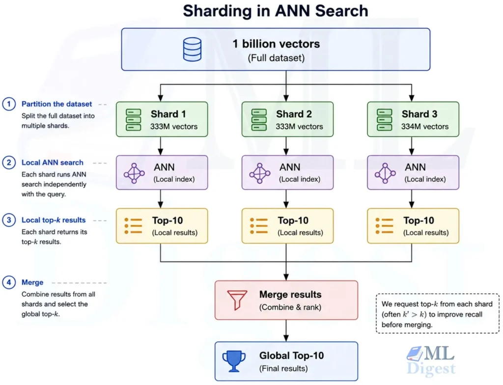
- Sharding: split the corpus across multiple shards, run ANN per shard, then merge the top-$k$ across shards.
- Replication: replicate shards to scale QPS and reduce tail latency.
- Batching: many libraries can process multiple queries in a batch more efficiently than one-by-one.
- Warm start and persistence: persist the index to disk, then measure load time, memory-mapping behavior, and warmup effects.
- Fallbacks: if the ANN service is degraded, decide whether to (a) return fewer results, (b) route to a slower exact service on a smaller subset, or (c) return cached results.
8. Minimal Python Walkthrough
This section shows a small end-to-end workflow. Treat it as a learning baseline, not as a benchmark configuration.
8.1 Create a toy dataset and exact baseline
import numpy as np

rng = np.random.default_rng(0)

n = 50_000
d = 128

X = rng.normal(size=(n, d)).astype(np.float32)
Q = rng.normal(size=(100, d)).astype(np.float32)

def l2_normalize(a: np.ndarray, eps: float = 1e-12) -> np.ndarray:
    norms = np.linalg.norm(a, axis=1, keepdims=True)
    return a / np.maximum(norms, eps)

# Example: cosine similarity via inner product after normalization
Xn = l2_normalize(X)
Qn = l2_normalize(Q)

def exact_topk_ip(X: np.ndarray, q: np.ndarray, k: int = 10):
    # Inner product similarity: larger is better.
    scores = X @ q

    # argpartition uses a 0-based "kth" position; use k-1 to get top-k.
    idx = np.argpartition(-scores, k - 1)[:k]
    idx = idx[np.argsort(-scores[idx])]
    return idx, scores[idx]

idx0, scores0 = exact_topk_ip(Xn, Qn[0], k=10)
print(idx0[:5], scores0[:5])
# My experimental output:
# [15607 44866 46355 26 41708] [0.34744686 0.33640078 0.3360735 0.32727584 0.32615495]This produces an exact top-$k$ result that can serve as ground truth when computing Recall@k.
8.2 Exact kNN with scikit-learn (baseline for small to medium scale)
from sklearn.neighbors import NearestNeighbors

k = 10

nn = NearestNeighbors(n_neighbors=k, algorithm="brute", metric="cosine")
nn.fit(Xn)

dist, ind = nn.kneighbors(Qn)
print(ind[0][:5], dist[0][:5])
# My experimental output:
# [15607 44866 46355 26 41708] [0.6525531 0.66359925 0.6639266 0.67272425 0.673845 ]Notes:
metric="cosine"returns cosine distance, so smaller values are more similar.- At large $n$, exact brute-force search becomes expensive.
8.3 HNSW with hnswlib (practical ANN starting point)
Install:
pip install hnswlibBuild and query:
import hnswlib

dim = Xn.shape[1]
num_elements = Xn.shape[0]

p = hnswlib.Index(space="cosine", dim=dim)
p.init_index(max_elements=num_elements, ef_construction=200, M=16)

# IDs are required; here we use 0..n-1
p.add_items(Xn, np.arange(num_elements))

# Trade-off knob for query time
p.set_ef(50)  # higher -> better recall, slower queries

labels, distances = p.knn_query(Qn, k=10)
print(labels[0][:5], distances[0][:5])
# My experimental output:
# [ 26 41708 35488 14255 46692] [0.6727241 0.673845 0.6894313 0.70186806 0.7026087 ]To compute Recall@k:
def recall_at_k(exact_idx: np.ndarray, ann_idx: np.ndarray, k: int) -> float:
    exact_set = set(exact_idx[:k].tolist())
    ann_set = set(ann_idx[:k].tolist())
    return len(exact_set & ann_set) / float(k)

q = Qn[0]
exact_idx, _ = exact_topk_ip(Xn, q, k=10)
ann_idx = labels[0]
print("Recall@10:", recall_at_k(exact_idx, ann_idx, k=10))
# My experimental output:
# Recall@10: 0.28.4 FAISS for scalable similarity search
FAISS is a similarity-search toolkit, not a separate ANN family. It provides exact indexes and several ANN families behind a consistent API, which makes it useful for comparing baselines and progressively trading quality for speed or memory.
| Retrieval goal | Typical FAISS index | Main trade-off |
|---|---|---|
| Exact reference results | IndexFlatL2 or IndexFlatIP | Scores every vector; simple and high quality, but expensive at scale. |
| High recall with available RAM | IndexHNSWFlat | Graph memory and construction time for strong recall-latency performance. |
| Fewer candidates, full-precision scoring | IndexIVFFlat | nprobe controls the recall-latency trade-off. |
| Large collection with tight memory | IndexIVFPQ | Compact codes reduce memory and scan cost, but add quantization error. |
For cosine retrieval, normalize vectors and use an inner-product index, because FAISS ranks inner products in descending order. IVF and PQ indexes must be trained with representative vectors before data is added. FAISS can also move supported indexes to GPUs, but CPU and GPU measurements should be compared separately because transfer, batching, and available memory affect the result.
FAISS supports exact flat indexes, graph indexes, IVF, PQ, and hybrid variants on CPU and, for many index types, GPU. Its main value is not a single algorithm but the ability to evaluate these alternatives with a common API. IVF-PQ is a common FAISS choice when collection size and memory use dominate the design.
Install (CPU):
pip install faiss-cpu8.4.1 Minimal IVF example (inner product / cosine)
At scale, IVF with inner product is a practical starting point. To use cosine similarity in FAISS, L2-normalize vectors and then use inner product.
import numpy as np
import faiss

# Xn, Qn from the earlier example are already L2-normalized float32 arrays.
dim = Xn.shape[1]

nlist = 1024   # number of coarse clusters (inverted lists)
nprobe = 10    # number of lists searched per query
k = 10

# Quantizer defines the coarse space; IndexFlatIP works well.
quantizer = faiss.IndexFlatIP(dim)
index = faiss.IndexIVFFlat(quantizer, dim, nlist, faiss.METRIC_INNER_PRODUCT)

# Train on a representative sample (required for IVF indices).
train_size = min(200_000, Xn.shape[0])
index.train(Xn[:train_size])

# Add database vectors.
index.add(Xn)

index.nprobe = nprobe
scores, ids = index.search(Qn, k)
print(ids[0][:5], scores[0][:5])
# My experimental output:
# [15607 9423 38136 7564 18242] [0.3474469 0.29032785 0.28760397 0.27464515 0.26697677]8.4.2 Minimal IVF-PQ example
IndexIVFPQ follows the same train, add, and search workflow as IndexIVFFlat, but stores a PQ code for every indexed vector rather than the full vector. Choose $m$ so that it divides the embedding dimension, and set nbits=8 for 256 codewords per sub-quantizer.
pq_quantizer = faiss.IndexFlatIP(dim)
m = 16        # number of sub-quantizers; must divide dim
nbits = 8     # bits per sub-quantizer, so 256 codewords

pq_index = faiss.IndexIVFPQ(
  pq_quantizer,
  dim,
  nlist,
  m,
  nbits,
  faiss.METRIC_INNER_PRODUCT,
)

# Training learns both the coarse IVF centroids and PQ codebooks.
pq_index.train(Xn[:train_size])
pq_index.add(Xn)

pq_index.nprobe = nprobe
scores, ids = pq_index.search(Qn, k)
print(ids[0][:5], scores[0][:5])
# My experimental output:
# [15607 2839 37385 38136 18242] [0.33925888 0.30940974 0.300505 0.29086196 0.28836262]The default code size here is $m \times \frac{\mathrm{nbits}}{8} = 16$ bytes per vector, excluding IVF-list and index overhead. Increasing $m$, nbits, or nprobe can improve recall, while increasing memory, build cost, or query latency.
Practical FAISS details
- Use
IndexIDMaporIndexIDMap2when application IDs are not simply0through $n-1$. - Persist a CPU index with
faiss.write_indexand load it withfaiss.read_index; measure load time and warmup in the serving environment. - Retain full vectors separately when exact reranking is required, because a PQ code alone cannot reconstruct an exact similarity score.
9. Practical Tips and Best Practices
The following practices have an outsized effect on retrieval quality and operational stability.
9.1 Normalize and validate your metric assumptions
- For cosine similarity, normalize both indexed vectors and queries.
- Ensure that the query-time embedding model, preprocessing, and metric match those used to build the index.
- Validate score direction explicitly: L2 is minimized, while inner product and cosine similarity are maximized.
9.2 Use a two-stage retrieval pattern when quality matters
A robust production template:
- ANN retrieves $R$ candidates (for example, $R=100$ to $R=2000$).
- Rerank exactly (full distance) or with a learned model.
- Return top $k$.
This lets ANN optimize candidate recall rather than perfect ordering in the final top $k$.
9.3 Tune parameters with a sweep, not by intuition
Keep the query set, machine type, concurrency, and measurement procedure fixed during a sweep so that results are comparable.
9.4 Plan for filtering and multi-tenancy early
Filtering changes the search problem.
- If you need hard filters (tenant, language, category), you have options:
- separate indices per segment
- hybrid: pre-filter candidates by metadata then ANN
- post-filter: ANN first then filter (can hurt recall if filters are selective)
The appropriate choice depends on filter selectivity, dataset size, and the index’s native filtering support. Measure recall after filtering, not only before it.
9.5 Monitor and refresh indices
Embedding distributions drift with: new data, model updates, domain shifts.
These shifts are the same family of data drift and concept drift tracked elsewhere in the ML lifecycle, so existing MLOps monitoring workflows can often be reused for the retrieval index.
Recommended controls:
- rebuild or retrain the index on an appropriate schedule
- version embeddings, model artifacts, index parameters, and evaluation data, for example with an experiment-tracking tool such as MLflow
- run offline evaluation and controlled online experiments when changing the embedding model or index configuration
9.6 Treat ANN tuning as a recall–latency budget allocation
If the end-to-end pipeline includes rerankers, filters, personalization, or business rules, ANN is only one part of the latency budget. A useful discipline is:
- Decide a p95 budget for retrieval.
- Tune ANN until Recall@$R$ is acceptable within that budget.
- Allocate the remaining time to reranking and business logic, where it may have greater task-level impact.
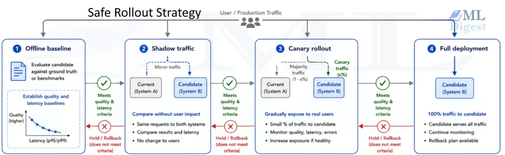
9.7 Use canaries and shadow traffic for safe changes
- ANN behavior can shift noticeably when you change: embedding model version, normalization logic, index hyperparameters, the library version or hardware.
Validate changes with:
- shadow traffic (evaluate new index without affecting users)
- canary rollout (small percentage of traffic)
- quality dashboards that include both retrieval metrics and task metrics
These validation habits follow the same discipline covered in testing machine learning code, applied here to a retrieval index instead of a model.
10. Common Pitfalls (And How to Avoid Them)
- Metric mismatch: L2 distance on embeddings intended for cosine similarity can invalidate retrieval results. Match normalization and score direction to the embedding model’s training and serving contract.
- Unrepresentative evaluation: a small or synthetic query set can conceal failure modes. Include real query distributions, difficult queries, and relevant metadata filters.
- Offline over-tuning: a configuration that wins a static benchmark can fail under production concurrency, distribution shift, or hardware constraints. Re-measure in a realistic serving environment.
- Ignoring tail latency: a fast median can still violate an interactive service-level objective. Track p95 and p99, particularly during index reloads and traffic spikes.
- Deletes and churn: frequent deletions or replacement of embeddings can degrade some indexes. Define compaction, rebuild, and rollback procedures before launch.
Closing Perspective
ANN is not a one-time library choice. It is an empirical systems decision: define the retrieval objective, measure exact ground truth, tune against a realistic latency budget, and keep validating as embeddings, traffic, and data change. A simple HNSW or IVF baseline with a disciplined evaluation protocol is usually more valuable than a sophisticated index that has not been measured on the workload it must serve.

Happy is a seasoned ML professional with over 15 years of experience. His expertise spans various domains, including Computer Vision, Natural Language Processing (NLP), and Time Series analysis. He holds a PhD in Machine Learning from IIT Kharagpur and has furthered his research with postdoctoral experience at INRIA-Sophia Antipolis, France. Happy has a proven track record of delivering impactful ML solutions to clients. Check more about him here: https://sites.google.com/site/slhappyin/

Silpa brings 5 years of experience in working on diverse ML projects, specializing in designing end-to-end ML systems tailored for real-time applications. Her background in statistics (Bachelor of Technology) provides a strong foundation for her work in the field. Silpa is also the driving force behind the development of the content you find on this site.
Subscribe to our newsletter!