Paper: A ConvNet for the 2020s (Liu et al., 2022), ConvNeXt V2
ConvNeXt modernizes the classic convolutional neural network (CNN) by applying the design principles and training techniques popularized by Vision Transformers (ViTs). Instead of introducing self-attention or complex new operations, it systematically upgrades a standard ResNet.
The result is a pure, highly practical ConvNet that is simple to implement and matches modern Transformer performance on vision benchmarks. This write-up walks through the modernization roadmap, explains the block-level mathematical formulation, and provides runnable PyTorch code.
1. The Question ConvNeXt Answers
The ConvNeXt paper asks a deceptively simple question:
If we update a ResNet with the design and training lessons learned from Transformers, how far can a pure ConvNet go?
The answer, as the paper demonstrates systematically, is: surprisingly far. If you have ever looked at the ViT wave and assumed convolution had been permanently sent to the retirement home, then ConvNeXt is the paper that proves otherwise.
Vision Transformers (ViTs) had achieved impressive results, and hierarchical variants like Swin Transformer extended those gains to dense prediction tasks like detection and segmentation. The common narrative was that the performance gap came from self-attention, a fundamentally new inductive bias. ConvNeXt challenges that narrative. It shows that much of the gap was due to training recipes and block design choices that had never been applied to ConvNets before.
2. Intuition: Modernizing the CNN
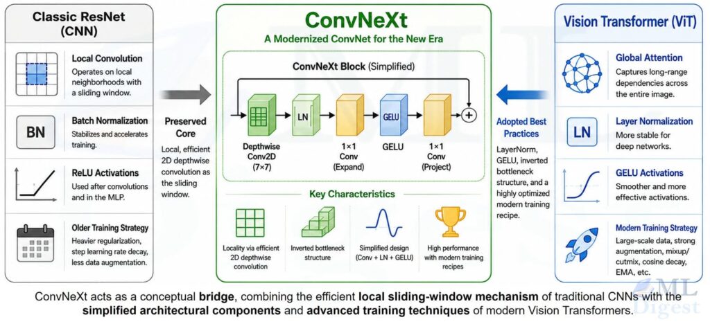
Think of ResNet-era ConvNets and Vision Transformers as representing two different design philosophies.
Classic ConvNets (ResNet) are highly reliable and optimized for local pattern recognition. However, many of their design conventions (such as where to place activation layers or which normalization to use) were shaped by older hardware limitations and training habits rather than modern best practices.
Vision Transformers (ViTs) utilize a clean, highly standardized block structure combined with powerful training recipes. Their minimalist approach and lack of historical baggage allowed them to quickly outperform classic architectures.
ConvNeXt bridges this gap. It preserves the efficiency of convolutional layers while adopting the simplified architecture and modern training strategy of Transformers. Rather than introducing a single complex breakthrough, ConvNeXt succeeds through a series of practical, empirically proven upgrades.
3. The Modernization Roadmap
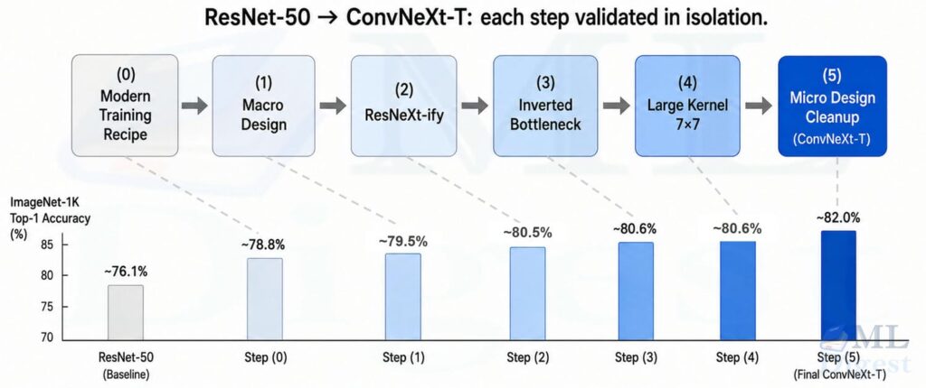
The paper transforms a standard ResNet-50 into ConvNeXt through a sequence of steps, measuring accuracy at each stage. Here is that journey:
3.1 Step 0: Modern Training Recipe
Before touching the architecture, the paper retrains ResNet-50 with a modern “DeiT-style” recipe: AdamW optimizer, Mixup and CutMix augmentation, RandAugment policies, stochastic depth (DropPath), Label Smoothing, and a longer 300-epoch schedule. This alone lifts ResNet-50 accuracy from roughly 76.1% to around 78.8% on ImageNet-1K.
That is the first humbling moment in the paper. Sometimes the flashy architectural debate is really a boring spreadsheet problem wearing sunglasses. A significant portion of the perceived Transformer advantage was simply a training recipe advantage.
3.2 Step 1: Macro Design
Two macro-level changes are made to align with Swin Transformer (as highlighted in below image):
- Stage ratio: The distribution of blocks across the four stages is changed from the classic ResNet pattern
(3, 4, 6, 3)to(3, 3, 9, 3), placing more compute in the third stage. - Patchify stem: The classic ResNet stem (a 7×7 convolution followed by max pooling) is replaced by a single stride-4 convolution, analogous to the patch embedding in ViT. This produces a cleaner, non-overlapping downsampling at the entry of the network.
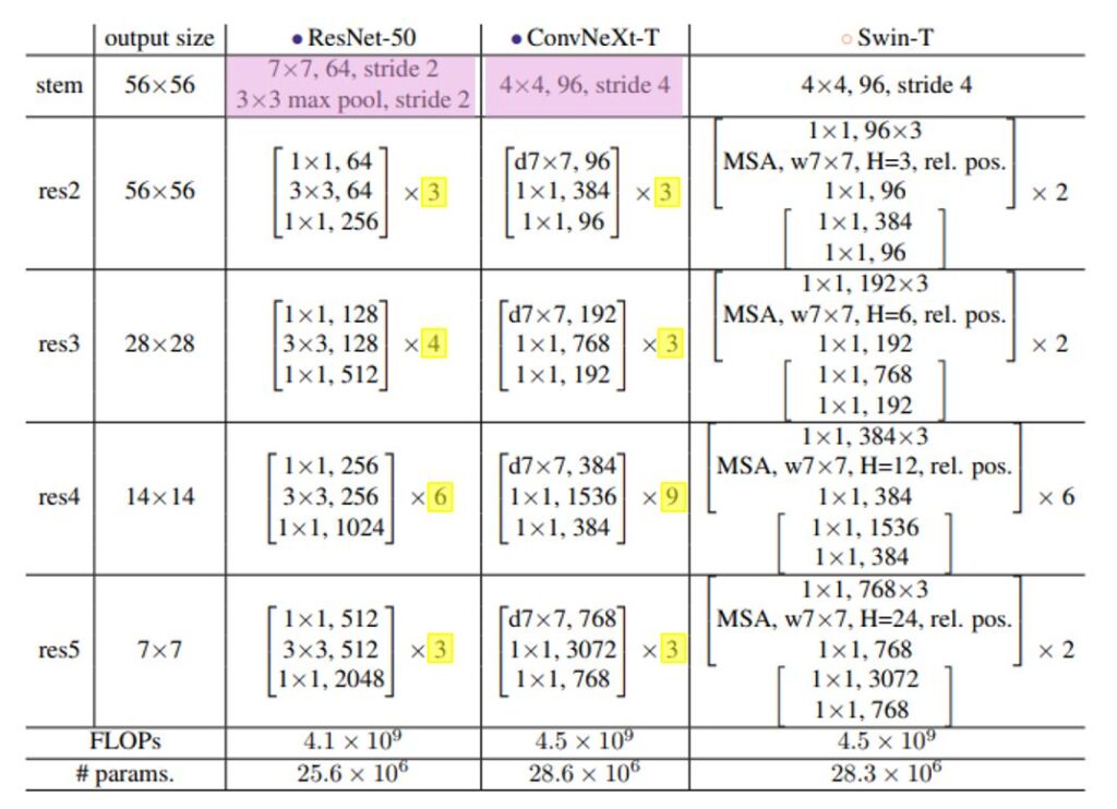
3.3 Step 2: ResNeXt-ify
The standard 3×3 convolutions in the main block are replaced with depthwise convolutions, where each filter operates on a single channel (groups = channels). This drastically reduces FLOPs, freeing capacity to increase the channel width and bring the overall model compute back to the original budget. This is the same depthwise trick popularized by MobileNet and Xception.
3.4 Step 3: Inverted Bottleneck
In a classic ResNet bottleneck, channels are squeezed (narrow in the middle). In a Transformer FFN (feed-forward network), channels are expanded in the middle. ConvNeXt flips to the inverted bottleneck: the pointwise (1×1) convolutions expand the channel count by a factor of four, apply a nonlinearity, and then project back. This mirrors the Transformer FFN design philosophy exactly.
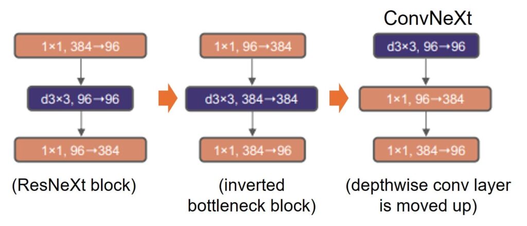
3.5 Step 4: Large Kernel Depthwise Convolution
As can be seen in above image, the position of the depthwise convolution is moved up, which mimics the self-attention’s position in the Transformer before the MLP layers. This helps in reducing the FLOPs. However, this resulted in a slight degradation in accuracy, but it was a necessary step to enable the next change: increasing the kernel size.
The depthwise convolution kernel size is increased from 3×3 to 7×7. This enlarges the effective receptive field at low cost (depthwise means the added FLOPs are minimal) and brings the local mixing operation closer in spirit to the broader context modeling of self-attention. The 7×7 size was chosen empirically; larger sizes provided diminishing returns.
If 3×3 kernels are the neural-network equivalent of peeking through a keyhole, 7×7 is at least opening the door a bit wider.
3.6 Step 5: Micro Design Cleanup
Finally, a set of small but impactful changes are made to each block:
- ReLU to GELU: The smoother Gaussian Error Linear Unit (GELU) activation, standard in Transformer models, replaces ReLU.
- Fewer activations and norms: ResNet blocks have multiple activations and normalization layers. ConvNeXt reduces to exactly one GELU and one LayerNorm per block, matching Transformer block simplicity.
- BatchNorm to LayerNorm: Batch Normalization is replaced with Layer Normalization everywhere.
- Separate downsampling layers: Downsampling is handled by dedicated layers rather than being embedded within the main block.
Each of these five steps contributes measurably, and together they produce the ConvNeXt block. The methodical progression is the point: Transformer performance is not magic; it is largely the product of these compounding modernization choices.
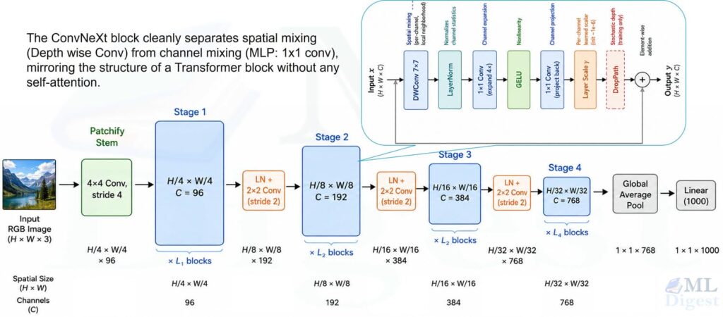
4. Inside the ConvNeXt Block
The ConvNeXt block is the paper’s main idea in one unit: use convolution for spatial mixing, then a Transformer-style channel MLP, then add the result back through a residual path.
4.1 Block Structure
At a single stage, ConvNeXt repeatedly applies the following residual unit:
- Depthwise convolution (7×7 kernel, one filter per channel)
- LayerNorm (normalizes over the channel dimension, applied per spatial position)
- Pointwise conv (1×1) expanding channels by 4x
- GELU activation
- Pointwise conv (1×1) projecting back to the original channel count
- Layer scale (learnable per-channel scalar, initialized to a very small value such as $10^{-6}$)
- DropPath (stochastic depth, applied during training)
- Residual addition with the input $x$
The skip path is identity. The main path performs wide local mixing, normalizes the result, applies a 4x channel MLP, rescales it with layer scale, optionally drops it during training, and adds it back. Initializing layer scale near zero makes the residual branch start as a small correction, which helps optimization.
In compact math, the block computes:
$$
\mathbf{y} = \mathbf{x} + \mathrm{DropPath}\left(\gamma \odot \mathrm{MLP}\left(\mathrm{LN}\left(\mathrm{DWConv}_{7\times7}(\mathbf{x})\right)\right)\right)
$$
where $\mathrm{MLP}(\cdot)$ denotes the two-layer pointwise stack, $\gamma \in \mathbb{R}^C$ is the per-channel layer-scale vector, and $\odot$ is broadcast element-wise multiplication over spatial dimensions.
4.2 Why Depthwise 7×7?
A depthwise convolution applies one spatial filter per channel, so a larger kernel stays cheap. At each spatial position, a 7×7 depthwise convolution over $C$ channels costs $49C$ multiply-adds, while a dense 7×7 convolution costs $49C^2$.
The wider kernel gives each location more local context before the channel MLP acts. It is still local, not global and input-adaptive like self-attention, but it is substantially less myopic than a 3×3 block.
4.3 LayerNorm vs. BatchNorm
ConvNeXt replaces BatchNorm with LayerNorm. BatchNorm depends on batch statistics, which can become brittle with small batches, transfer learning, or distribution shift.
LayerNorm instead normalizes within each sample across channels at each spatial position. That makes the behavior batch-size independent and aligns ConvNeXt with standard Transformer practice.
In PyTorch, nn.LayerNorm expects the last dimension, so implementations often use channels-last layout (N, H, W, C) internally, or permute around the normalization step when the rest of the model uses (N, C, H, W).
4.4 The Inverted Bottleneck and Transformer Analogy
The two 1×1 convolutions form an inverted bottleneck: expand channels by 4x, apply GELU, then project back down. This is the convolutional analogue of the Transformer feed-forward network.
| Transformer FFN | ConvNeXt Block |
|---|---|
| Linear expand (4x) | 1×1 conv expand (4x) |
| GELU | GELU |
| Linear project | 1×1 conv project |
This is why ConvNeXt feels Transformer-like even without attention: spatial mixing first, channel MLP second, residual wrapper last. The difference is the mixer itself. Self-attention is content-adaptive and global; depthwise convolution is fixed-form and local.
4.5 Why the Hierarchical Design Matters
The block is only half the story. ConvNeXt is also hierarchical: spatial resolution shrinks while channel width grows across stages.
This differs from isotropic architectures such as the original ViT, where token grid and embedding width stay mostly fixed. For detection and segmentation, multi-scale features are usually more useful.
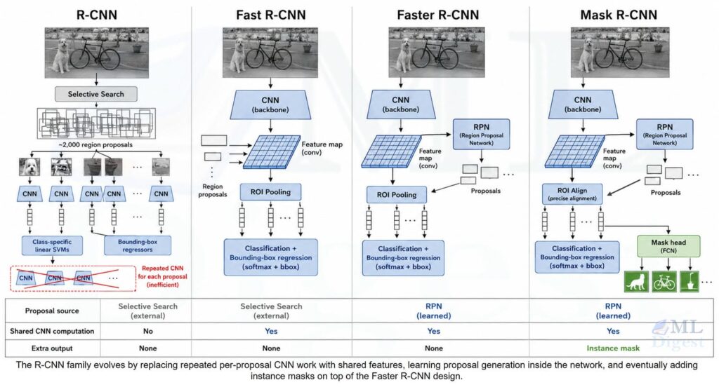
Because ConvNeXt reduces resolution stage by stage, it naturally exposes a feature pyramid at strides 4, 8, 16, and 32. That makes it a near drop-in replacement for ResNet in pipelines such as Mask R-CNN and Cascade R-CNN, and it also slots naturally into DETR-family transformer-based detectors as a CNN backbone.
Stage Layout and Downsampling
Between stages, spatial resolution is halved and channel count is doubled. Each transition uses an explicit downsampling module:
LayerNorm -> Conv(Ci, Ci+1, kernel=2, stride=2)Keeping downsampling outside the main block makes the repeated residual unit cleaner and more modular.
4.6 Model Variants
ConvNeXt scales by stage depth and width. The paper provides five standard sizes:
| Model Variant | Channels (C) | Blocks (B) | FLOPs (G) | Params (M) |
|---|---|---|---|---|
| ConvNeXt-T (Tiny) | (96, 192, 384, 768) | (3, 3, 9, 3) | 4.5 | 28 |
| ConvNeXt-S (Small) | (96, 192, 384, 768) | (3, 3, 27, 3) | 8.7 | 50 |
| ConvNeXt-B (Base) | (128, 256, 512, 1024) | (3, 3, 27, 3) | 15.4 | 89 |
| ConvNeXt-L (Large) | (192, 384, 768, 1536) | (3, 3, 27, 3) | 34.4 | 198 |
| ConvNeXt-XL (Extra Large) | (256, 512, 1024, 2048) | (3, 3, 27, 3) | 60.9 | 350 |
The (3, 3, 27, 3) layout in the larger variants mirrors Swin’s stage allocation, which makes compute-matched comparisons easier to read and helps position ConvNeXt as a full backbone family rather than a one-off tweak.
5. Training Recipe: The Other Half of the Story
The training recipe is not a footnote; it is central to ConvNeXt’s results. The paper emphasizes that architecture and training choices are entangled, and comparing old ConvNet recipes to modern Transformer recipes is not a fair comparison.
I think this is one of the healthiest lessons in the paper. It pushes you away from architecture tribalism and toward cleaner experimental thinking. If one model got a personal trainer, better food, and eight extra hours of sleep, you do not get to call the comparison fair.
The modern recipe ConvNeXt uses includes:
- Optimizer: AdamW with decoupled weight decay (the standard Transformer optimizer choice, not SGD with momentum).
- Data augmentation: RandAugment-style policies, Mixup, and CutMix.
- Regularization: stochastic depth (DropPath) and label smoothing.
- Schedule: cosine decay with a linear warmup period, extended training budget (300 epochs for a fair comparison).
- EMA: exponential moving average of weights, often beneficial for final model quality.
The practical lesson is this: if you benchmark a ResNet trained with an older recipe against ConvNeXt trained with a stronger recipe, you will incorrectly attribute training gains to architecture. ConvNeXt is a package, and the two halves reinforce each other.
6. ConvNeXt V2: Masked Pretraining and Global Response Normalization
In 2023, the same authors released ConvNeXt V2, which addresses one remaining limitation: masked autoencoder (MAE) style self-supervised pretraining.
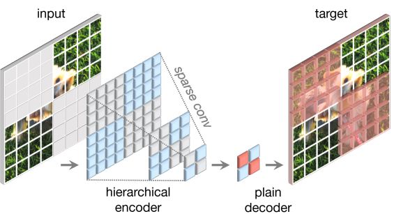
6.1 The Problem with MAE and Dense ConvNets
MAE pretrains a model by masking random patches of the image and asking the encoder to reconstruct them. With ViTs, masking is clean: you simply remove patch tokens from the sequence. With dense ConvNets, masking is harder because convolution operations can “see around” masked patches through overlapping receptive fields, allowing information leakage.
ConvNeXt V2 solves this with a Fully Convolutional Masked Autoencoder (FCMAE): during pretraining, sparse convolution processes only the visible patches, preventing any leakage from masked regions. This makes masked pretraining efficient and principled for ConvNets.
6.2 Global Response Normalization (GRN)
Sparse pretraining revealed a second problem: feature collapse. With intense, varied masking, feature maps can become saturated or collapse to redundant representations.
ConvNeXt V2 adds a Global Response Normalization (GRN) layer inside each block, after the GELU activation. GRN computes a global descriptor from each feature channel by aggregating across spatial dimensions, and uses it to re-scale the channel activations, increasing the contrast between channels and reducing redundancy.
The operation is:
$$
Gx_c = |X_c|_2, \quad Nx_c = \frac{Gx_c}{\mathrm{mean}(\mathbf{Gx}) + \epsilon}
$$
$$
\mathrm{GRN}(X) = \gamma \odot (X \odot \mathbf{Nx}) + \beta + X
$$
where $Gx_c$ is the L2 norm of channel $c$ aggregated over the spatial $(H, W)$ dimensions, $\mathbf{Nx}$ re-scales each channel relative to the mean channel norm (increasing contrast between channels), and $\gamma, \beta \in \mathbb{R}^C$ are learnable per-channel scalars initialized to zero. The residual $+X$ ensures GRN starts as an identity at initialization, which stabilizes early training under masked pretraining.
The result: ConvNeXt V2-Base achieves 84.9% ImageNet-1K top-1 accuracy, compared to 83.8% for V1-Base at the same scale.
7. Implementation: What to Watch For
A few gotchas that frequently cause confusion:
- Channels-last layout: reference implementations use
(N, H, W, C)internally for LayerNorm efficiency. When integrating with other code that uses the standard(N, C, H, W)layout, you need explicit permutations or a wrapper. The PyTorchto(memory_format=torch.channels_last)call handles this at the model level. - Layer scale initialization: the layer scale $\gamma$ must be initialized to a very small value (typically $10^{-6}$). This is not cosmetic. It makes the residual branch contribute almost nothing at the start of training, which stabilizes optimization in deeper models. This connects to broader weight initialization principles — initialization choices profoundly affect whether training converges or diverges, particularly given the vanishing gradient problem that destabilizes deep networks at initialization.
- Explicit downsamplers: do not hide the stride-2 downsampling inside the main block. Use a separate LayerNorm + stride-2 conv module at each stage transition, matching the paper.
- Stochastic depth rates: use increasing drop rates with depth. Deeper blocks get higher drop probability. This is important for larger variants.
- Kernel size: the 7×7 depthwise kernel is a meaningful ingredient. Reducing it to 3×3 noticeably hurts accuracy, as shown in the paper’s ablation.
8. Code Examples
The timm library provides reference ConvNeXt implementations for both inference and fine-tuning.
8.1 Inference with a Pretrained ConvNeXt
This example loads a pretrained ConvNeXt-Tiny and runs inference:
import torch
import timm  # pip install timm


def main():
    # Load a pretrained ConvNeXt-Tiny from the timm model zoo
    model = timm.create_model("convnext_tiny", pretrained=True)
    model.eval()

    # Standard ImageNet input: batch of 1 RGB image at 224x224
    x = torch.randn(1, 3, 224, 224)

    with torch.no_grad():
        logits = model(x)

    # logits shape: [1, 1000] for ImageNet-1K
    print("logits shape:", logits.shape)

    probs = logits.softmax(dim=-1)
    top5 = torch.topk(probs, k=5, dim=-1)
    print("top-5 class indices:", top5.indices[0].tolist())
    print("top-5 probabilities: ", [f"{v:.4f}" for v in top5.values[0].tolist()])


if __name__ == "__main__":
main()Note: if you are on Windows and need GPU support, use the official PyTorch install selector to get the CUDA-enabled build.
8.2 Fine-Tuning on a New Task
This example adapts a pretrained ConvNeXt-Tiny to a 10-class classification problem. It is intentionally minimal (no dataloader), but captures the settings that matter most in practice:
import torch
import timm


def build_model(num_classes: int = 10) -> torch.nn.Module:
    # pretrained=True loads ImageNet weights; num_classes replaces the head
    model = timm.create_model("convnext_tiny", pretrained=True, num_classes=num_classes)
    return model


def example_train_step(model: torch.nn.Module, device: str = "cpu") -> float:
    model.to(device)
    model.train()

    # channels_last layout aligns with how LayerNorm is most efficiently applied
    model = model.to(memory_format=torch.channels_last)

    # Dummy batch: 8 images at 224x224
    x = torch.randn(8, 3, 224, 224, device=device).to(
        memory_format=torch.channels_last
    )
    y = torch.randint(0, model.num_classes, (8,), device=device)

    # AdamW + label smoothing matches the ConvNeXt training recipe
    optimizer = torch.optim.AdamW(model.parameters(), lr=1e-4, weight_decay=0.05)
    criterion = torch.nn.CrossEntropyLoss(label_smoothing=0.1)

    logits = model(x)
    loss = criterion(logits, y)

    optimizer.zero_grad(set_to_none=True)
    loss.backward()
    optimizer.step()

    return float(loss.detach().cpu())


if __name__ == "__main__":
    model = build_model(num_classes=10)
print("training loss:", example_train_step(model))Practical tips aligned with the paper:
- Use AdamW with a cosine learning rate schedule and a short linear warmup when fine-tuning more than just the classification head.
- Keep DropPath (stochastic depth) active when using deeper variants (ConvNeXt-B and above).
- Preserve layer scale. Removing it destabilizes training in deep models.
- With small batch sizes (below 32), LayerNorm makes fine-tuning less brittle than with BatchNorm-heavy backbones.
9. ConvNeXt vs. Vision Transformers: When to Choose Which
Neither architecture dominates universally. The right choice depends on your task and constraints.
ConvNeXt holds several practical advantages. Its strong inductive biases (locality and translation equivariance) help when training data is limited, and convolution kernels are aggressively optimized on modern hardware (NVIDIA GPUs, Apple Silicon, and edge accelerators), making inference efficient. At comparable FLOPs budgets, it consistently outperforms earlier CNN families such as EfficientNet. It is also a near-direct drop-in replacement for ResNet in any pipeline with a standard feature pyramid neck, and it integrates smoothly with existing deployment tooling such as ONNX, TensorRT, and CoreML.
Vision Transformers have different strengths. Self-attention can directly connect distant image regions without deep stacking, making it better suited for tasks that require flexible global context. Larger pretraining regimes (CLIP-scale or MAE-scale) tend to favor attention-based models, and isotropic ViTs adapt more naturally to non-image modalities such as audio, video, and 3D point clouds treated as sequences. Multi-modal transformers have extended this versatility further, handling vision, language, audio, and video in unified architectures.
As a practical heuristic: if you want a strong vision backbone for a task where ResNet already worked, ConvNeXt is likely a direct upgrade with predictable behavior. If you are working with very large pretraining datasets or need flexible global context modeling, a strong ViT (such as ViT-L/14 or a CLIP vision encoder) may serve better. Vision-language models such as BLIP similarly rely on ViT-based encoders for their vision component, given the flexibility that global attention provides across cross-modal tasks.
Summary
ConvNeXt demonstrates that the perceived performance gap between ResNets and Vision Transformers was not primarily about self-attention. It was about a collection of design and training choices that Transformers happened to get right first.
The core contributions are:
- A systematic modernization roadmap from ResNet to ConvNeXt, with each step empirically validated.
- A block that implements the Transformer philosophy (spatial mixing then channel mixing, with LayerNorm and residuals) entirely in convolution.
- A training recipe aligned with what modern Transformer training uses.
ConvNeXt V2 extends this with masked-pretraining compatibility and Global Response Normalization.
For practitioners, ConvNeXt is one of the most accessible routes to strong vision performance: it fits familiar ConvNet tooling, scales predictably, and transfers well. Start with convnext_tiny from timm, swap it in wherever you have a ResNet backbone, and iterate from there.
Common Questions
Does ConvNeXt use any form of attention?
No. ConvNeXt is a purely convolutional model. The Transformer-inspired improvements come from block layout, normalization choice, and training recipe, not from adding attention layers.
Is ConvNeXt just a ResNet with bigger kernels?
Not exactly. Kernel size is an important ingredient, but ConvNeXt also changes the normalization (LayerNorm), the stem and downsampling strategy, the bottleneck orientation (inverted), activation type (GELU), and the training recipe. Any single change alone produces modest gains; the combination is what closes the gap.
Does ConvNeXt show that Transformers are unnecessary for vision?
No, and the paper does not claim this. The result is more nuanced: ConvNets were not fundamentally limited by convolution. They were limited by older design choices and training practices. Once updated, they become competitive. Both paradigms remain strong, and the best choice is context-dependent.
What changed in ConvNeXt V2 versus V1?
Two things: (1) FCMAE pretraining, which uses sparse convolution to enable masked-patch self-supervised learning without information leakage; (2) Global Response Normalization (GRN), added to the block to prevent feature collapse during sparse training. Together these improvements raise accuracy by roughly 0.5-1.0% across model sizes.

Happy is a seasoned ML professional with over 15 years of experience. His expertise spans various domains, including Computer Vision, Natural Language Processing (NLP), and Time Series analysis. He holds a PhD in Machine Learning from IIT Kharagpur and has furthered his research with postdoctoral experience at INRIA-Sophia Antipolis, France. Happy has a proven track record of delivering impactful ML solutions to clients.
Subscribe to our newsletter!