Paper: DINO: Emerging Properties in Self-Supervised Vision Transformers (Caron et al., 2021), DINOv2: Learning Robust Visual Features without Supervision (Oquab et al., 2023)
Think of supervised learning as teaching a child with flashcards: this is a cat, this is a dog, this is a car. DINO takes a different route. It is closer to showing the child the same scene through multiple windows and asking, “What stays meaningfully the same?” If the model can answer that question consistently, it starts to build useful visual understanding without any human labels.
That idea made DINO one of the most influential self-supervised learning methods for Vision Transformers (ViTs). DINOv2 kept the same teacher-student intuition, then turned it into a stronger visual pretraining system with curated data, better large-scale stability, and features that are practical to reuse as frozen backbones.
This write-up explains what DINO is optimizing, why it works so well with ViTs, what changed in DINOv2, and how practitioners typically use the resulting features.
1. Why DINO Mattered
Before DINO, self-supervised learning in vision was already moving fast, but many methods depended on carefully designed contrastive losses, very large negative batches, or training tricks that were difficult to stabilize. DINO showed that a simpler teacher-student distillation setup could learn strong visual features without labels, and it worked especially well with Vision Transformers.
Its importance comes from three observations:
- It learns semantic image representations without manual annotation.
- It works unusually well with ViTs, often producing attention maps that align with objects.
- It turns a pretrained encoder into a reusable backbone for classification, retrieval, segmentation, and dense matching.
In practice, DINO helped shift the field toward the idea that a vision encoder could be pretrained once and reused broadly across tasks.
2. Intuition: What DINO Is Really Teaching the Model
At a high level, DINO trains a student network to match the output of a teacher network when both see different views of the same image.
Imagine an image of a bicycle. One crop shows the full bicycle, another shows only the wheel, another shows the frame plus part of the background. The teacher sees large, global crops. The student sees both global and local crops. The training signal says: even if the student sees only a part of the object, it should still produce a representation compatible with what the teacher inferred from the broader scene.
That forces the network to learn features that are consistent across augmentations, sensitive to semantics rather than pixel identity, and useful beyond a single downstream task.
A Mental Picture: The Classroom Analogy
A helpful way to picture DINO is as a classroom with one calm teacher and one fast-learning student.
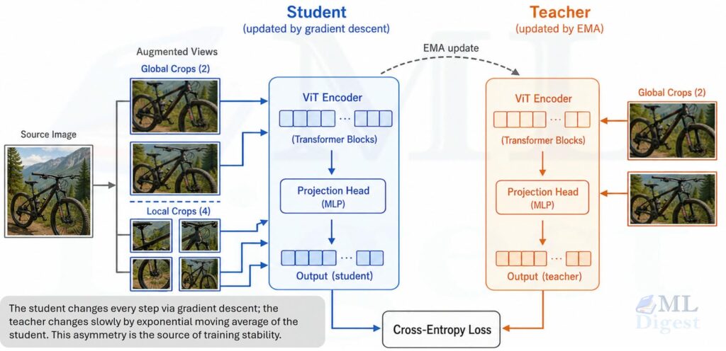
As shown in the figure, the teacher sees only global crops, while the student sees both global and local crops. The student is trained to match the teacher’s output across all view pairings. The teacher is updated as a slow-moving average of the student, which provides a stable target for the student to chase.
The slow teacher acts like a stable reference point. That stability is one reason DINO avoids collapse without relying on explicit negative pairs.
The data flow works in three stages:
- One image is split into two large global crops and several small local crops.
- The teacher receives only the global crops; the student receives all of them.
- The student outputs are trained to match the teacher outputs across all view pairings.
The central directive is to match the meaning, not the pixels. Applied consistently across views, this constraint drives the model toward semantic representations.
3. DINO Architecture and Training Pipeline
DINO uses two networks with the same architecture, usually a Vision Transformer:
- a student network with parameters $\theta_s$,
- a teacher network with parameters $\theta_t$.
Both networks process augmented views of the same image. Their encoder outputs are passed through projection heads that map features into a probability distribution over prototypes.
3.1 Multi-Crop Augmentation
One of DINO’s most important design choices is multi-crop training. The teacher receives only a few global views with large spatial coverage, while the student receives both those global views and several local views with small crops.
Why does that matter? The student must align a partial observation with a fuller one, which pushes the representation toward object-level and scene-level consistency. Without this asymmetry, the model has little reason to encode anything beyond low-level texture.
3.2 Student and Teacher Outputs
Let $x$ be an image view. After the encoder and projection head, the student produces logits $g_{\theta_s}(x)$ and the teacher produces logits $g_{\theta_t}(x)$. These logits are converted into probability distributions:
$$
P_s(x) = \operatorname{softmax}\left(\frac{g_{\theta_s}(x)}{\tau_s}\right)
$$
$$
P_t(x) = \operatorname{softmax}\left(\frac{g_{\theta_t}(x) – c}{\tau_t}\right)
$$
where $\tau_s$ is the student temperature, $\tau_t$ is the teacher temperature, and $c$ is a running center used to stabilize teacher outputs.
The centering and sharpening steps are central to DINO’s training stability.
3.3 Centering and Sharpening
Without labels, the easiest bad solution is collapse: the model maps every image to nearly the same representation.
DINO counters this with two opposing forces that work together.
Centering spreads the teacher output away from dominating dimensions. The center $c$ is updated as an exponential moving average of teacher outputs:
$$
c \leftarrow \lambda c + (1 – \lambda) \cdot \frac{1}{B}\sum_{i=1}^{B} g_{\theta_t}(x_i)
$$
Sharpening makes teacher predictions peaky enough to carry information. This is controlled by the low teacher temperature $\tau_t$.
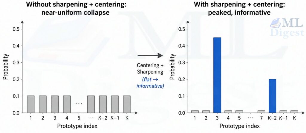
This is a simple idea with a large practical effect. It reduces collapse pressure while remaining lighter-weight than methods that depend on large-batch contrastive structure.
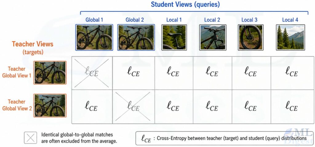
3.4 Cross-View Self-Distillation Loss
For teacher view $x$ and student view $x’$, DINO minimizes the cross-entropy between teacher and student distributions:
$$
\mathcal{L}(x, x’) = – \sum_{k=1}^{K} P_t^{(k)}(x) \log P_s^{(k)}(x’)
$$
where $K$ is the number of output prototypes.
The full loss averages across different view pairings of the same image, typically excluding pairings of identical global crops:
$$
\mathcal{L}_{\text{DINO}} = \frac{1}{|\mathcal{P}|} \sum_{(x, x’) \in \mathcal{P}} \mathcal{L}(x, x’)
$$
The key insight is subtle but important: the model is not reconstructing pixels and not matching labels. It is matching the teacher’s semantic distribution across views. That objective, applied across many images and many crops, is what drives the features toward semantic structure.
3.5 EMA Teacher Update
The teacher is not updated by backpropagation. Instead, it is an exponential moving average of the student:
$$
\theta_t \leftarrow m \, \theta_t + (1 – m) \, \theta_s
$$
where $m$ is a momentum coefficient, often annealed upward during training (starting around 0.996 and ending near 1.0).
This means the teacher is a smoother, more temporally stable version of the student. Stability is a major part of why DINO works: the student is chasing a target that changes slowly, which prevents feedback loops from destabilizing training.
4. Why DINO Works So Well with Vision Transformers
DINO can be trained with convolutional neural networks, but it became especially notable because of what happened with ViTs. ViTs split an image into patches and process them as tokens, maintaining a single unified resolution throughout—a key structural difference from hierarchical architectures like the Swin Transformer that progressively downsample feature maps across stages. In DINO-pretrained ViTs, the self-attention maps often align surprisingly well with foreground objects or coherent semantic regions.
That led to one of the memorable findings of the original work: useful object localization behavior can emerge even without labels.
Why is that plausible? Patch tokens preserve spatial structure naturally. Cross-view consistency encourages the model to find the stable semantic parts. Multi-crop training forces local patches to answer to global context. The combination naturally directs attention toward the semantically stable regions of an image.
4.1 Self-Attention Alignment with Objects
A well-known finding from the original DINO paper is that the CLS token’s self-attention maps tend to localize foreground objects rather than spreading uniformly across the image.
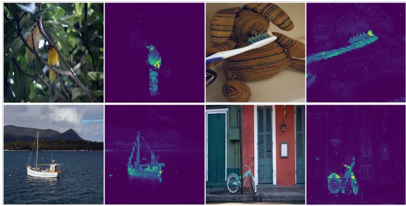
 (Image source: DINO paper; DINO’s self-attention learns to localize foreground objects without any spatial supervision. This emergent property follows from cross-view consistency: the network attends to image parts whose meaning is stable across crops.)
Visualizing those maps for an image of a bird shows the model attending to the animal’s body and largely ignoring background regions, despite no spatial annotations ever being provided. This emergent localization is one of the clearest qualitative signs that the model is learning more than image-level shortcuts.
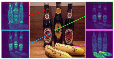 (Image source: DINO paper)
As can be seen in the figure above, the self-attention maps are not just focused on one part of the image. Different reference points attend to different parts of the object, which suggests that the model is learning a rich internal representation of the object’s structure.
4.2 Strengths and Limitations of Original DINO
Strengths
- Strong transfer learning with linear probing and k-nearest-neighbor evaluation.
- No human labels required for pretraining.
- Particularly effective for ViT feature learning.
- Produces useful patch-level structure even when trained from an image-level objective.
Limitations
- Training stability becomes harder at larger scale.
- Performance depends strongly on augmentations and recipe details.
- The original DINO was powerful, but not yet a complete all-purpose visual foundation model on the scale practitioners wanted.
- Dense tasks such as depth and segmentation benefited from the learned features, but the method was not designed from the start as a scaled universal frozen-feature pipeline.
These limitations are exactly where DINOv2 enters.
5. DINOv2 at a High Level
DINOv2 is best understood as a scaled and production-minded successor to DINO. It keeps the mean-teacher, self-distillation core, but strengthens nearly every surrounding component: data curation, training stability, local-feature learning, model scaling, and deployment into smaller distilled checkpoints.
The result is a family of pretrained ViTs that produce robust features usable out of the box across many image-level and pixel-level tasks.
The central promise of DINOv2 is straightforward: train a very strong visual encoder on a very large curated image collection, then reuse its frozen features directly with lightweight heads or nearest-neighbor methods.
This matters because many vision pipelines become simpler when the backbone stays fixed. Training is cheaper, debugging is easier, and the same representation can serve several downstream tasks.
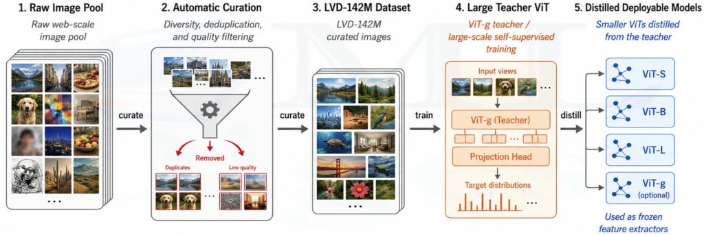
5.1 Curated Large-Scale Data
DINOv2 was trained on LVD-142M, a curated dataset of 142 million images assembled from a much larger uncurated pool. The curation step is important. The authors did not simply collect more images; they built an automatic pipeline to keep the data diverse and useful while reducing redundancy and low-value noise.
That design choice is one of the biggest differences between a strong research recipe and a useful foundation-model pipeline.
5.2 Larger Teachers, Distilled Smaller Students
DINOv2 trains very large ViTs, including a roughly one-billion-parameter ViT-g model, then distills that knowledge into smaller variants such as ViT-S, ViT-B, and ViT-L. Those distilled models remain much easier to deploy while retaining a large share of the representational quality.
This follows a recurring pattern in modern ML systems: use a very large model to learn the best representation possible, then compress it into smaller models through knowledge distillation for actual deployment.
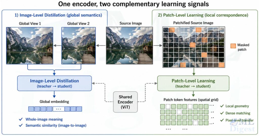
5.3 Image-Level Plus Patch-Level Learning
Original DINO is centered around image-level self-distillation. DINOv2 builds on DINO and iBOT-style masked patch prediction so that training also learns stronger local features.
This matters because many downstream tasks need more than a single global embedding:
- Depth estimation needs local geometry.
- Semantic segmentation needs spatially aligned patch features.
- Dense matching needs correspondences between parts.
DINOv2 is therefore not only better at saying “these two images are similar.” It is also better at saying “these local regions correspond semantically.”
5.4 DINOv2 Training Objective in Plain Language
At a high level, DINOv2 combines an image-level self-distillation loss in the style of DINO, a patch-level learning objective inspired by iBOT, and additional regularization and systems choices that make large-scale training stable and efficient.
The image-level objective teaches global semantics; the patch-level objective teaches local structure; the regularization and data pipeline make both scale more reliably.
Conceptual Decomposition
If we write the total objective schematically:
$$
\mathcal{L}_{\text{total}} = \mathcal{L}_{\text{image}} + \alpha \, \mathcal{L}_{\text{patch}} + \beta \, \mathcal{L}_{\text{reg}}
$$
where:
- $\mathcal{L}_{\text{image}}$ is the DINO-style image-level cross-view distillation loss,
- $\mathcal{L}_{\text{patch}}$ is a masked patch objective for local tokens; this is often implemented as a cross-entropy loss over masked patches, similar to iBOT,
- $\mathcal{L}_{\text{reg}}$ represents additional regularization for stable, well-spread features,
- $\alpha$ and $\beta$ are scalar weighting hyperparameters.
The exact recipe includes several implementation details, but the conceptual message is enough for most practitioners: DINOv2 learns both the whole picture and the pieces of the picture.
In the paper, that regularization includes mechanisms such as feature-space spreading terms, often discussed through the KoLeo regularizer, whose job is not to inject semantics but to keep the representation from collapsing into a narrow part of feature space.
5.5 Why DINOv2 Was a Major Step Forward
DINOv2 demonstrated that self-supervised, image-only pretraining can compete with, and on most of the paper’s reported image-level and pixel-level benchmarks surpass, image-text systems such as CLIP, BLIP, and related OpenCLIP variants for pure visual representation quality.
That is important because caption-based supervision has a structural blind spot: captions often mention only a few semantic facts and omit rich local structure. An image encoder trained only through text alignment may therefore under-emphasize fine-grained spatial information. DINOv2, by learning directly from image structure, often produces features that are especially strong for dense visual tasks.
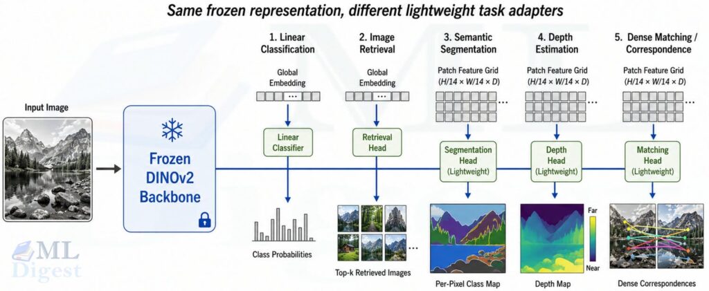
The frozen features from DINOv2 show strong performance across a wide range of tasks:
- Image classification with linear probing
- Instance retrieval
- Dense matching and patch correspondence
- Semantic segmentation with lightweight heads
- Monocular depth estimation
- Video understanding through frame-level feature reuse
One of the strongest practical messages from DINOv2 is this: frozen features can already be very good, which reduces the need for expensive full-model fine-tuning.
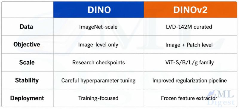
6. DINO vs. DINOv2
| Aspect | DINO | DINOv2 |
|---|---|---|
| Core idea | Self-distillation with no labels | Scaled self-distillation foundation model |
| Main supervision | Image-level cross-view distillation | Image-level and patch-level learning |
| Scale | Strong research method | Large curated-data foundation model |
| Data | Smaller curated setups such as ImageNet-scale pretraining | LVD-142M curated web-scale dataset |
| Model family | Mainly research checkpoints | Distilled deployable family from ViT-S to ViT-g |
| Best use today | Understanding SSL ideas, reproducing research, custom pretraining | Off-the-shelf visual feature extraction |
The short version: DINO is the idea; DINOv2 is the mature system.
7. Implementation Details That Practitioners Should Care About
If you are using these models rather than reproducing the original papers, a few details matter much more than the full theory.
7.1 Use DINOv2 as a Frozen Feature Extractor First
In many practical pipelines, the best starting point is:
- Extract global embeddings from the class token for image-level tasks.
- Extract patch embeddings for dense tasks.
- Train only a shallow downstream head.
This is simpler, faster, and often surprisingly competitive with full fine-tuning. The official DINOv2 repository, PyTorch Hub interface, and Hugging Face model collection all support this workflow directly.
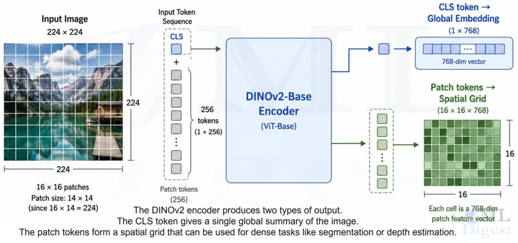
7.2 Match the Patch Grid to Your Task
DINOv2 models commonly use a patch size of 14. That means the hidden states can be split into one global token and a grid of local patch tokens. For dense tasks, those patch tokens are often more valuable than the class token alone.
If the patch-grid arithmetic feels abstract, it helps to review how Vision Transformer tokens are computed and how positional embeddings encode spatial ordering before wiring those features into a downstream head.
7.3 Expect Strong Zero-Shot Structure, Not Magic Labels
DINOv2 features are powerful, but they are still visual embeddings, not a full multimodal reasoning system. They excel at structure, similarity, locality, and transfer. They do not automatically give task-specific labels unless you add a head or another retrieval or classification mechanism.
7.4 Useful Resources Before You Build
If you want to move from reading to hands-on use, three resources cover most practical needs:
- The paper for the training recipe and benchmark context.
- The Meta AI blog post for the high-level motivation and deployment framing.
- The demo and model card for quick inspection of features and inference behavior.
7.5 Pseudocode for DINO-Style Training
Before looking at production code, it helps to understand the training loop in plain pseudocode. The following captures the core logic without boilerplate.
for images in dataloader:
    global_views, local_views = make_multi_crop_views(images)

    # Teacher sees only global crops; student sees everything
    teacher_views = global_views
    student_views = global_views + local_views

    teacher_logits = [teacher(view) for view in teacher_views]
    student_logits = [student(view) for view in student_views]

    # Sharpen teacher with low temperature; center to prevent collapse
    teacher_probs = [sharpen_and_center(logits, center=c, tau=tau_t)
                     for logits in teacher_logits]
    # Soften student with higher temperature
    student_probs = [softmax(logits / tau_s) for logits in student_logits]

    # Average cross-entropy over all (teacher, student) view pairs
    loss = 0.0
    num_terms = 0
    for teacher_out in teacher_probs:
        for student_out in student_probs:
            loss += cross_entropy(teacher_out, student_out)
            num_terms += 1
    loss = loss / num_terms

    optimizer.zero_grad()
    loss.backward()        # only updates the student
    optimizer.step()

    # Update running center and EMA teacher
    update_center(teacher_logits, center=c, momentum=lambda_c)
ema_update(student, teacher, momentum=m)The important pieces are not the exact helper functions. The important pieces are: multi-view augmentation, stable teacher targets, EMA teacher update, and cross-view prediction. Everything else is engineering around those four ideas.
8. Runnable Code: Feature Extraction with DINOv2
The most practical code example today is feature extraction rather than training DINO from scratch. The snippet below uses Hugging Face Transformers to load the facebook/dinov2-base checkpoint and separate global and patch features. It downloads a sample image from the COCO dataset so the example stays reproducible.
import torch
import requests
from PIL import Image
from transformers import AutoImageProcessor, AutoModel


def load_image(url: str) -> Image.Image:
    """Download and convert an image to RGB."""
    response = requests.get(url, stream=True, timeout=30)
    response.raise_for_status()
    return Image.open(response.raw).convert("RGB")


def main() -> None:
    # Load a sample image from the COCO validation set
    image = load_image("http://images.cocodataset.org/val2017/000000039769.jpg")

    # Load the pretrained DINOv2-Base processor and model
    processor = AutoImageProcessor.from_pretrained("facebook/dinov2-base")
    model = AutoModel.from_pretrained("facebook/dinov2-base")
    model.eval()

    # Preprocess: resize, normalize, and batch the image
    inputs = processor(images=image, return_tensors="pt")

    with torch.no_grad():
        outputs = model(**inputs)

    # last_hidden_state shape: (batch, 1 + num_patches, hidden_dim)
    hidden = outputs.last_hidden_state

    # Token 0 is the CLS token: the global image summary
    cls_embedding = hidden[:, 0, :]         # (1, 768)

    # Tokens 1: are the patch tokens: local spatial features
    patch_embeddings = hidden[:, 1:, :]     # (1, num_patches, 768)

    # Reshape flat patch sequence back to a spatial grid
    batch_size, _, image_height, image_width = inputs["pixel_values"].shape
    patch_size = model.config.patch_size    # 14 for dinov2-base
    num_patches_h = image_height // patch_size
    num_patches_w = image_width // patch_size

    # patch_grid shape: (1, H/14, W/14, 768)
    patch_grid = patch_embeddings.unflatten(1, (num_patches_h, num_patches_w))

    print("Pixel tensor:       ", inputs["pixel_values"].shape)
    print("Last hidden state:  ", hidden.shape)
    print("Global CLS embedding:", cls_embedding.shape)
    print("Patch grid:         ", patch_grid.shape)


if __name__ == "__main__":
main()What This Code Is Doing
cls_embeddingis the global image representation, useful for retrieval or linear classification.patch_gridis a spatial tensor of local features, useful for segmentation, matching, or saliency-style analysis.
This is one reason DINOv2 is so practical: a single backbone gives both a whole-image summary and a dense feature map.
Typical Next Steps After Feature Extraction
Once you have these features, common downstream patterns include:
- Training a linear classifier on
cls_embeddingfor image classification. - Running k-nearest-neighbor retrieval over a database of embeddings.
- Clustering patch embeddings for rough unsupervised segmentation.
- Feeding patch features into a lightweight depth or segmentation head.
9. Practical Tips and Best Practices
When to Choose DINOv2: Use DINOv2 when you want strong general-purpose visual embeddings, a frozen backbone that can serve several tasks, patch-level features for dense vision, or minimal dependence on text supervision.
When Original DINO Is Still Worth Studying: Study DINO directly when you want to understand the mechanics of non-contrastive SSL, to implement a research reproduction, or to pretrain on a custom domain with a more interpretable and controllable training setup.
Common Mistakes: Several mistakes come up frequently when people first work with these models:
- Treating the class token as the only useful output. For dense tasks, patch tokens often matter more, or even exclusively.
- Comparing DINOv2 only on classification. Some of its strongest behavior shows up in retrieval, depth, and dense matching.
- Assuming self-supervised means no downstream data is ever needed. The backbone can be frozen, but many applications still benefit from a small supervised head.
- Ignoring data quality. DINOv2’s gains are not only about architecture. Data curation was a major part of the advance; it is not simply “more data.”
A Simple Way to Remember Both Models
If you need a compact mental model:
- DINO teaches a model to agree with itself across views.
- DINOv2 scales that idea into a robust visual foundation model by improving data, objectives, and distillation.
Another way to say it:
- DINO asks, “Can two views of the same image lead to the same meaning?”
- DINOv2 asks, “Can that principle produce universal visual features at foundation-model scale?”
The answer to the second question is largely yes, and that is why DINOv2 remains one of the most useful image-only pretrained backbones in modern computer vision. If you are starting a new vision project today and want reliable frozen features, DINOv2 is one of the first checkpoints worth evaluating.

Happy is a seasoned ML professional with over 15 years of experience. His expertise spans various domains, including Computer Vision, Natural Language Processing (NLP), and Time Series analysis. He holds a PhD in Machine Learning from IIT Kharagpur and has furthered his research with postdoctoral experience at INRIA-Sophia Antipolis, France. Happy has a proven track record of delivering impactful ML solutions to clients.

Silpa brings 5 years of experience in working on diverse ML projects, specializing in designing end-to-end ML systems tailored for real-time applications. Her background in statistics (Bachelor of Technology) provides a strong foundation for her work in the field. Silpa is also the driving force behind the development of the content you find on this site.
Subscribe to our newsletter!