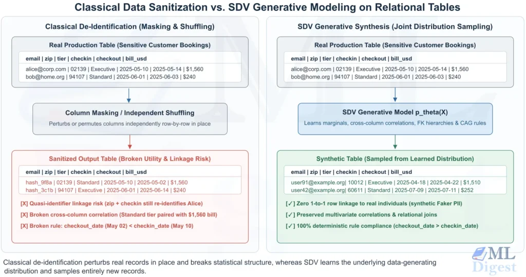
Building reliable machine learning models and software tests often requires realistic data, yet data privacy laws (GDPR, HIPAA, CCPA) can restrict access to personal data. De-identification methods such as masking, hashing, shuffling, or $k$-anonymity have different privacy and utility trade-offs: depending on implementation, they can leave re-identification risks or disrupt useful correlations and joins.
The Synthetic Data Vault (SDV) brings synthetic data generation to structured data by fitting generative models over the statistical patterns, relational hierarchies, and temporal dynamics of real tables and sampling entirely new records. Originating at MIT’s Data to AI Lab, SDV covers single-table synthesis (GaussianCopulaSynthesizer, CTGANSynthesizer, TVAESynthesizer), multi-table relational databases (HMASynthesizer), sequential time series (PARSynthesizer), business-rule enforcement (sdv.cag), and quality evaluation (SDMetrics).
Why Tabular and Relational Synthesis Is Uniquely Difficult
Unlike homogeneous text sequences or pixel grids in image, enterprise relational databases introduce five structural challenges that break standard neural architectures:
- Heterogeneous Semantic Data Types (
sdtypes): Single tables mix continuous floats, discrete integers, high-cardinality strings, ordered ranks, timestamps, booleans, and formatted identifiers (UUIDs, postal codes, emails). - Non-Gaussian and Multimodal Continuous Distributions: Real-world numerical columns exhibit heavy skew, sharp bounds, and multiple modes. Standard min-max or $z$-score normalization causes vanishing gradients or mode collapse in neural generators.
- Severe Categorical Imbalance: Categorical attributes frequently follow power-law distributions where rare classes (such as fraud or rare diagnoses) constitute less than $2\%$ of rows, starving standard mini-batch training and compounding downstream imbalanced data challenges.
- Deterministic Business Logic: Records must obey strict invariants, such as $\mathrm{checkout_date} > \mathrm{checkin_date}$, $\mathrm{total_price} = \mathrm{subtotal} + \mathrm{tax} – \mathrm{discount}$, or valid $(\mathrm{country}, \mathrm{currency})$ pairs.
- Relational Referential Integrity: Normalized databases require preserving both internal table distributions and cross-table properties, including degree distributions (child rows per parent) and cross-table correlations across foreign keys.
| Data Sanitization Strategy | Privacy Protection | Cross-Column Correlation | Multi-Table Referential Integrity | Deterministic Business Rules | Rare Edge-Case Simulation |
|---|---|---|---|---|---|
| Static Masking / Hashing | Low (linkage attacks) | Destroyed on masked fields | Preserved if deterministic | Broken on dates and totals | Impossible |
| $k$-Anonymity / Binning | Moderate to High | Degraded by generalization | Degraded across joins | Degraded by bucketing | Suppressed as outliers |
Rule-Based (Faker) | High (no real data used) | None (independent columns) | Manual scripting required | Manual rules required | Manual specification |
| Synthetic Data Vault (SDV) | High (samples from distribution) | Preserved via joint modeling | Preserved via HMASynthesizer | Enforced via sdv.cag | Supported via Condition |
Architectural Overview of the SDV Ecosystem
SDV is structured as a modular stack coordinated around a declarative Metadata contract. The SDV package is distributed under a Business Source License; check the terms of each component and edition rather than assuming the entire stack is open source:
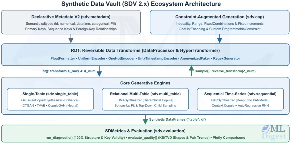
Each sub-package in the sdv-dev organization handles one stage of the generative lifecycle:
sdv.metadata: Declares the structural and semantic schema of tables (METADATA_SPEC_VERSION = "V2").- RDT (Reversible Data Transforms): Encodes heterogeneous columns (dates, strings, booleans, missing values, and PII) into numerical vectors before fitting, and inverts the transformation during sampling.
- Copulas: Implements multivariate statistical copula models that decouple univariate marginals from inter-column dependency structures.
- CTGAN: Implements PyTorch-based deep generative tabular models (
CTGANandTVAE). - DeepEcho: Implements Probabilistic AutoRegressive (
PAR) neural networks for variable-length multi-entity time-series synthesis. - SDMetrics: Computes diagnostic checks, statistical similarity scores, and Plotly visual comparisons between real and synthetic datasets.
Phase 1: Metadata and Reversible Data Transforms (RDT)
Rather than relying on raw pandas storage dtypes (int64, object, float64), SDV classifies each column by its semantic data type (sdtype):
Semantic Type (sdtype) | Role in Synthesis | Default RDT Transformer (Statistical / Copula) | Default RDT Transformer (Deep Learning / CTGAN) |
|---|---|---|---|
id | Primary, foreign, or sequence keys | AnonymizedFaker (keys; RegexGenerator if regex_format is set; UniformEncoder for non-keys) | AnonymizedFaker (keys; RegexGenerator if regex_format is set; OneHotEncoder for non-keys) |
numerical | Continuous or discrete quantities | FloatFormatter (rounding, bounds, null flag) | FloatFormatter + ClusterBasedNormalizer (variational GMM) |
datetime | Timestamps and dates | UnixTimestampEncoder (epoch conversion) | UnixTimestampEncoder + ClusterBasedNormalizer |
categorical | Unordered discrete labels | UniformEncoder (frequency intervals) | OneHotEncoder (feeds softmax/Gumbel outputs) |
ordinal | Ordered discrete levels | OrderedUniformEncoder (preserves rank order) | OneHotEncoder |
boolean | Binary True / False flags | UniformEncoder | OneHotEncoder |
PII (email, name, ssn, etc.) | Sensitive fields excluded from fitting | AnonymizedFaker (Faker-generated values at sample time) | AnonymizedFaker |
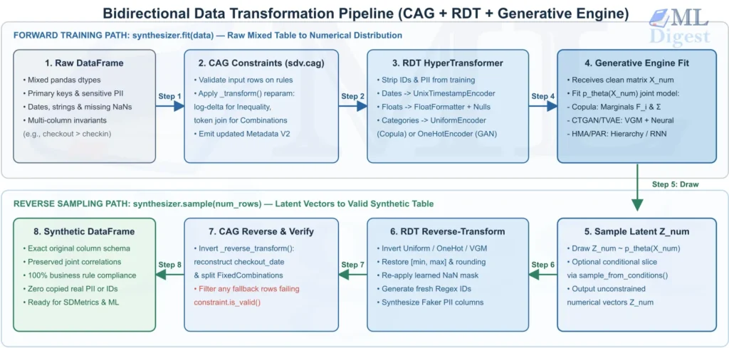
SDV coordinates preprocessing and postprocessing through DataProcessor and rdt.HyperTransformer:
Continuous Encoding of Discrete and Numerical Columns
Because statistical copulas operate strictly in continuous space, RDT’s UniformEncoder maps a categorical column $C$ with $K$ categories ${c_1, \dots, c_K}$ and empirical frequencies $p_k = P(C = c_k)$ onto contiguous sub-intervals $[a_k, b_k] \subseteq [0, 1]$:
$$a_k = \sum_{j=1}^{k-1} p_j, \qquad b_k = \sum_{j=1}^{k} p_j = a_k + p_k$$
During transform(), each observation $C = c_k$ is mapped to a continuous value $u \in [a_k, b_k]$. During reverse_transform(), any sampled $\hat{u} \in [a_k, b_k]$ maps back to $c_k$.
For numerical columns, FloatFormatter records three properties during fit() and restores them during reverse_transform():
- Decimal precision: Rounding digits present in the real column.
- Boundary extrema: Observed
[min, max]bounds (enforced whenenforce_min_max_values=True). - Missingness: Configurable missing-value replacement and generation can use an indicator or random missingness; preservation of missingness correlations depends on the configuration.
Phase 2: Single-Table Generative Engines
SDV provides four single-table synthesizers under sdv.single_table, ranging from fast statistical copulas to deep neural networks.
1. GaussianCopulaSynthesizer: Statistical Dependency via Sklar’s Theorem
Powered by copulas, GaussianCopulaSynthesizer relies on Sklar’s Theorem to separate each column’s individual shape from the cross-column correlation structure:
$$F(x_1, \dots, x_d) = C\big(F_1(x_1), \dots, F_d(x_d)\big)$$
Fitting and sampling proceed in four intuitive steps:
- Fit Column Shapes: Estimate a 1D distribution $F_i$ for each column independently (such as Beta, Gamma, Truncated Normal, or Gaussian KDE) to capture skew and bounds.
- Project to Normal Space: Convert each column’s values into uniform percentiles $(0, 1)$ and map them onto a standard normal bell curve.
- Learn Cross-Column Correlations: Compute the covariance and correlation matrix $\Sigma$ across all normalized columns.
- Sample & Invert: Draw correlated normal vectors from $\mathcal{N}(\mathbf{0}, \Sigma)$, map them through the standard normal CDF to uniform values, and apply each marginal inverse $F_i^{-1}$.
GaussianCopulaSynthesizer trains in milliseconds on CPU, avoids neural mode collapse, and produces the compact parameter vectors needed for multi-table synthesis.
2. CTGANSynthesizer: Deep Generative Modeling for Imbalanced Tables
For complex non-linear interactions, CTGANSynthesizer implements Modeling Tabular Data using Conditional GAN (Xu et al., NeurIPS 2019). Standard Generative Adversarial Networks (GANs) struggle with multi-peaked numerical columns and rare categories. CTGAN solves both through three mechanisms:
- Mode-Specific Normalization: Instead of global min-max scaling,
CTGANfits a variational Gaussian Mixture Model (GMM) to each numerical column. Every value is encoded by its nearest cluster (mode) and its relative distance from that mode’s center, preserving multi-peaked distributions. - Training-by-Sampling: To prevent rare categories (such as fraud or rare diagnoses) from being ignored,
CTGANsamples discrete categories according to their log-frequency during training. It passes the selected category as a condition vector to the generator and penalizes mismatched outputs. - PacGAN Critic: Rather than judging one row at a time, the Wasserstein critic (WGAN-GP) inspects packs of
10rows jointly (PacGAN), making lack of diversity immediately visible and preventing mode collapse.
Architecturally, the generator stacks concatenation-based residual layers with batch normalization and mixed output activation functions (tanh for continuous mode scalars and Gumbel-Softmax for discrete indicators), while the critic applies LeakyReLU and dropout regularization.
3. TVAESynthesizer and CopulaGANSynthesizer
TVAESynthesizer(Tabular Variational Autoencoder): Combines mode-specific normalization with a Variational Autoencoder (VAE) trained using reconstruction loss and KL Divergence. Because it has no adversarial critic,TVAEtrains faster and more stably thanCTGAN, often achieving higher correlation accuracy on medium-sized tables (5,000to100,000rows).CopulaGANSynthesizer: Uses Gaussian Copula transformations to smooth heavy-tailed numerical columns into normal space before trainingCTGAN.
Phase 3: Multi-Table Relational Synthesis with HMA (HMASynthesizer)
Training separate models on a parent table (accounts) and a child table (invoices) breaks two relational properties:
- Cross-table correlations: Parent attributes (such as
plan_type = "Enterprise") strongly influence child values (such asamount_usd). - Child row counts (degree distribution): The number of child rows per parent varies systematically across parent records.
SDV’s Hierarchical Modeling Algorithm (HMASynthesizer) preserves both using a two-step bottom-up fit and top-down sample workflow:
Step 1: Bottom-Up Parameter Flattening (fit)
- Group by Parent Key: For each parent record, gather all of its linked child rows.
- Summarize Child Slice: Fit a local Gaussian Copula on that parent’s child rows and extract a flat summary vector containing:
- The number of child rows for that parent.
- Each child column’s distribution parameters (mean, spread, bounds).
- Pairwise correlations between the child columns.
- Augment Parent Table: Append these summary values as extra columns onto the parent row, then fit a root Gaussian Copula over the expanded parent table to learn how parent attributes and child distributions co-vary.
Step 2: Top-Down Conditional Reconstruction (sample)
- Sample Parent Rows: Generate synthetic parent rows—along with their synthetic child summary parameters—from the root model.
- Reconstruct & Sample Children: For each synthetic parent, rebuild a local child Gaussian Copula from its sampled parameters, generate the predicted number of child rows, and link them via the parent’s primary key.
Scaling Note: Because a child table with $m$ columns adds $\mathcal{O}(m^2)$ pairwise correlation columns to its parent,
HMASynthesizerraises aSynthesizerInputErroron schemas with more than5tables or a relationship depth greater than2(and definesMAX_NUMBER_OF_COLUMNS = 1000for augmented tables).
Phase 4: Sequential Time-Series Synthesis with PAR (PARSynthesizer)
Longitudinal datasets—such as sensor telemetry, patient vitals, or transaction histories—consist of multiple entities (sensor_id), each with static attributes (facility_zone) and a variable-length sequence of time-ordered measurements (reading_timestamp, temperature_c) commonly used in downstream time-series forecasting.
PARSynthesizer (powered by deepecho.PARModel) generates multi-entity time series in three steps:
- Model Static Context First: Collapses each entity’s constant attributes (
context_columns) and initial start time into one row per entity, fitting aGaussianCopulaSynthesizerto learn entity-level distributions. - Convert Timestamps to Step-by-Step Time Gaps: Replaces raw timestamps with step-by-step differences ($\Delta t_t = t_t – t_{t-1} \ge 0$, clipped to observed
[min, max]step bounds viaFloatFormatter). Summing these non-negative gaps from the sampled start time prevents time reversals during sampling. - Generate Sequences Autoregressively: Conditions a Recurrent Neural Network (RNN) on each entity’s sampled context vector. At each step $t$, the network predicts the next measurement’s distribution, the time gap $\Delta t_t$, and the probability of ending the sequence, producing realistic variable-length trajectories.
Phase 5: Constraint-Augmented Generation (sdv.cag)
Statistical fidelity is insufficient if generated rows violate deterministic business rules. SDV’s Constraint-Augmented Generation (sdv.cag) enforces multi-column invariants using reversible reparameterization before falling back to rejection sampling:
Constraint Class (sdv.cag) | Business Rule Enforced | Mathematical Reparameterization (_transform / _reverse_transform) |
|---|---|---|
Inequality | low_column_name <= high_column_name (or $<$ if strict_boundaries=True) | Replaces high_column with $\delta = \log(x_{\mathrm{high}} – x_{\mathrm{low}} + 1)$; reconstructs $\hat{x}_{\mathrm{high}} = \hat{x}_{\mathrm{low}} + (\exp(\hat{\delta}) – 1)$ at sample time. |
Range | low_column_name < middle_column_name < high_column_name (or $\le$ if strict_boundaries=False) | Replaces middle_column and high_column with $\delta_1 = \log(x_{\mathrm{mid}} – x_{\mathrm{low}} + 1)$ and $\delta_2 = \log(x_{\mathrm{high}} – x_{\mathrm{mid}} + 1)$, reconstructing $\hat{x}_{\mathrm{mid}}$ and $\hat{x}_{\mathrm{high}}$ sequentially via $\exp(\hat{\delta}) – 1$. |
FixedCombinations | Valid discrete column tuples (e.g., (city, country)) | Maps observed tuples to categorical lookup IDs (fixed_combination#k) in column city#country before fitting and restores tuples via lookup dictionary after sampling. |
FixedIncrements | Multiples of step $m$ (increment_value=5) | Divides by $m$ before fitting ($x’ = x / m$) and restores $\hat{x} = \mathrm{round}(\hat{x}’) \times m$ at sample time. |
OneHotEncoding | Exactly one binary indicator column in a group equals 1 | Maps binary columns to continuous values in ${\epsilon, 1 – \epsilon}$ (OHE#<col>) and sets the row-wise argmax column to 1 during sample() (or collapses to one categorical column when learning_strategy="categorical"). |
ProgrammableConstraint | Custom multi-column transformations and validations | Subclass interface exposing fit, transform, reverse_transform, is_valid, and get_updated_metadata. |
Chained Reparameterization vs. Reject Sampling Fallback
When registering rules via add_constraints() (sdv/single_table/base.py):
- Primary Path (
_chained_constraints): Applies constraints as forward transformations and updatesMetadata. SDV also validates candidates after reversing each transformation; first-draw acceptance is not guaranteed. - Fallback Path (
_reject_sampling_constraints): If a constraint cannot be chained but is compatible with the original metadata, SDV may validate it through rejection sampling. Sampling can require retries or fail to produce the requested number of rows.
Hands-On Python Implementation
Install SDV in your Python environment:
pip install sdv==2.2.0Single-Table Synthesis with Metadata V2, PII Anonymization, and Constraints
Metadata.detect_from_dataframes() infers semantic types (sdtype) from a dictionary of tables, allowing explicit PII configuration and sdv.cag constraint attachment before fitting:
import numpy as np
import pandas as pd
from sdv.cag import FixedCombinations, Inequality
from sdv.evaluation import evaluate_quality, run_diagnostic
from sdv.metadata import Metadata
from sdv.sampling import Condition
from sdv.single_table import CTGANSynthesizer, GaussianCopulaSynthesizer, TVAESynthesizer

# 1. Construct an illustrative hotel dataset with fake email addresses and business constraints
rng = np.random.default_rng(42)
n_rows = 600

checkin_dates = pd.to_datetime("2025-01-01") + pd.to_timedelta(
    rng.integers(0, 180, size=n_rows), unit="D"
)
stay_nights = rng.integers(1, 14, size=n_rows)
checkout_dates = checkin_dates + pd.to_timedelta(stay_nights, unit="D")

# Valid (room_tier, includes_lounge) pairs
tier_idx = rng.choice([0, 1, 2], size=n_rows, p=[0.60, 0.25, 0.15])
tiers = np.array(["Standard", "Deluxe", "Executive_Suite"])[tier_idx]
lounge = np.array(["No", "No", "Yes"])[tier_idx]
nightly_base = np.array([120.0, 210.0, 390.0])[tier_idx]
total_bill = np.round(stay_nights * nightly_base * rng.normal(1.0, 0.08, size=n_rows), 2)

guests_df = pd.DataFrame({
    "booking_id": [f"BK-{10000 + i}" for i in range(n_rows)],
    "guest_email": [f"guest_{i}@example.org" for i in range(n_rows)],
    "room_tier": tiers,
    "includes_lounge": lounge,
    "checkin_date": checkin_dates.strftime("%Y-%m-%d"),
    "checkout_date": checkout_dates.strftime("%Y-%m-%d"),
    "total_bill_usd": total_bill,
    "has_rewards": rng.choice([True, False], size=n_rows, p=[0.35, 0.65]),
})

# In SDV 2.x, all modalities pass a dictionary mapping table_name -> DataFrame
real_data = {"hotel_bookings": guests_df}

# 2. Auto-detect Metadata V2 and explicitly verify PII and primary key settings
metadata = Metadata.detect_from_dataframes(data=real_data)
metadata.update_column(
    column_name="booking_id",
    table_name="hotel_bookings",
    sdtype="id",
    regex_format="BK-[0-9]{5}",
)
metadata.update_column(
    column_name="guest_email",
    table_name="hotel_bookings",
    sdtype="email",
    pii=True,
)
for column in ("checkin_date", "checkout_date"):
    metadata.update_column(
        column_name=column,
        table_name="hotel_bookings",
        sdtype="datetime",
        datetime_format="%Y-%m-%d",
    )
metadata.set_primary_key(column_name="booking_id", table_name="hotel_bookings")
metadata.validate()
metadata.validate_data(data=real_data)

# 3. Initialize GaussianCopulaSynthesizer with custom marginal distributions
synthesizer = GaussianCopulaSynthesizer(
    metadata=metadata,
    enforce_min_max_values=True,
    enforce_rounding=True,
    numerical_distributions={"total_bill_usd": "gamma"},
)

# 4. Attach Constraint-Augmented Generation (CAG) rules
constraints = [
    Inequality(
        low_column_name="checkin_date",
        high_column_name="checkout_date",
        strict_boundaries=True,
    ),
    FixedCombinations(
        column_names=["room_tier", "includes_lounge"],
    ),
]
synthesizer.add_constraints(constraints=constraints)

# 5. Fit the synthesizer and sample 500 synthetic bookings
synthesizer.fit(data=real_data)
synthetic_data = synthesizer.sample(num_rows=500)
synthetic_bookings_df = synthetic_data["hotel_bookings"]

print(synthetic_bookings_df.head())Conditional Scenario Simulation (sample_from_conditions)
Conditional sampling generates targeted hypothetical slices—such as stress-testing a microservice on Executive_Suite reward members or augmenting rare records for fraud detection and anomaly detection—without requiring large real subsamples:
# Define hypothetical slices to synthesize
executive_reward_condition = Condition(
    num_rows=150,
    column_values={
        "room_tier": "Executive_Suite",
        "includes_lounge": "Yes",
        "has_rewards": True,
    },
)

standard_non_reward_condition = Condition(
    num_rows=150,
    column_values={
        "room_tier": "Standard",
        "includes_lounge": "No",
        "has_rewards": False,
    },
)

conditional_synthetic = synthesizer.sample_from_conditions(
    conditions=[executive_reward_condition, standard_non_reward_condition]
)
print(conditional_synthetic["hotel_bookings"]["room_tier"].value_counts())GaussianCopulaSynthesizer can condition mathematically in the transformed space, while CTGANSynthesizer uses rejection sampling for this public API. Constraints can require additional rejection sampling even for a copula. Rare or incompatible conditions may fail or yield fewer rows; see the conditional sampling guide.
HMASynthesizer does not currently support conditional sampling. PARSynthesizer has a separate sample_sequential_columns() interface for supplying context; do not assume the single-table conditional API applies to every modality. Consult the documentation for your installed version.
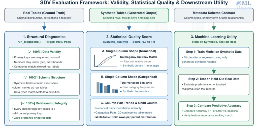
Phase 6: Quantitative Evaluation and Diagnostics (sdv.evaluation)
Complementary to pre-training data hygiene gates such as the Open-Source Dataset Validator, SDV integrates SDMetrics under sdv.evaluation through two core reports:
1. run_diagnostic(): Structural and Validity Checks (Target: $100\%$)
run_diagnostic(real_data, synthetic_data, metadata) evaluates applicable checks, rather than proving overall correctness or privacy:
- Data Validity: Checks key uniqueness and completeness, numerical bounds, and category adherence where applicable.
- Data Structure: Checks that the expected tables and columns are present.
- Relationship Validity: Checks referential integrity for applicable parent-child relationships.
- Constraint Validity: When constraints are supplied, checks the supported rules. A single-table dataset has no relationship property to evaluate.
2. evaluate_quality(): Statistical Fidelity Metrics ($0.0 \to 1.0$)
Much like statistical data drift detection between training and production splits, evaluate_quality(real_data, synthetic_data, metadata) scores selected distributional similarities between real and synthetic tables, including:
- Column Shapes (Univariate Marginal Fidelity):
- Continuous / Datetime: Kolmogorov-Smirnov (KS) Complement between real empirical CDF $F_{\mathrm{real}}(x)$ and synthetic CDF $F_{\mathrm{syn}}(x)$:
$$\mathrm{KSComplement} = 1 – \sup_{x} \big| F_{\mathrm{real}}(x) – F_{\mathrm{syn}}(x) \big| \in [0, 1]$$
- Categorical / Boolean: Total Variation Distance (TVD) Complement across categories $\Omega$:
$$\mathrm{TVComplement} = 1 – \frac{1}{2} \sum_{\omega \in \Omega} \big| P_{\mathrm{real}}(\omega) – P_{\mathrm{syn}}(\omega) \big| \in [0, 1]$$
- Column Pair Trends (Bivariate Dependency Fidelity):
- Numerical-Numerical: Compares real and synthetic correlation coefficients ($r_{\mathrm{real}}, r_{\mathrm{syn}}$).
CorrelationSimilaritysupports Pearson and Spearman; the report uses Pearson by default:
- Numerical-Numerical: Compares real and synthetic correlation coefficients ($r_{\mathrm{real}}, r_{\mathrm{syn}}$).
$$\mathrm{CorrelationSimilarity} = 1 – \frac{|r_{\mathrm{real}} – r_{\mathrm{syn}}|}{2} \in [0, 1]$$
- Categorical-Categorical: Contingency Similarity (2D Total Variation Complement between normalized contingency tables).
- Numerical-Categorical: Discretizes the numerical column into 10 equal-width histogram bins before computing 2D Contingency Similarity.
- Cardinality (Multi-Table Degree Fidelity): Compares child-row-count distributions per parent primary key via
KSComplement. - Intertable Trends: Multi-table reports can also compare relationships between columns across linked tables. These scores do not establish privacy or downstream utility.
from sdv.evaluation import (
    evaluate_quality,
    get_column_pair_plot,
    get_column_plot,
    run_diagnostic,
)

# 1. Run structural & validity diagnostics (Target: 1.0 / 100%)
diagnostic_report = run_diagnostic(
    real_data=real_data,
    synthetic_data=synthetic_data,
    metadata=metadata,
    constraints=[constraint.get_constraint_dict() for constraint in synthesizer.get_constraints()],
    verbose=True,
)

# 2. Run statistical quality evaluation (Column Shapes & Column Pair Trends)
quality_report = evaluate_quality(
    real_data=real_data,
    synthetic_data=synthetic_data,
    metadata=metadata,
    verbose=True,
)

print(f"Overall Quality Score: {quality_report.get_score():.4f}")
print(quality_report.get_details(property_name="Column Shapes"))

# 3. Generate interactive Plotly figures for univariate and bivariate inspection
fig_col = get_column_plot(
    real_data=real_data,
    synthetic_data=synthetic_data,
    metadata=metadata,
    table_name="hotel_bookings",
    column_name="total_bill_usd",
)
fig_pair = get_column_pair_plot(
    real_data=real_data,
    synthetic_data=synthetic_data,
    metadata=metadata,
    table_name="hotel_bookings",
    column_names=["room_tier", "total_bill_usd"],
)For downstream predictive tasks, pair evaluate_quality() with Machine Learning Efficacy (TSTR, Train on Synthetic, Test on Real): train tabular predictors such as XGBoost, LightGBM, or TabPFN on synthetic_data and evaluate classification metrics (ROC-AUC, $F_1$) on held-out real_data. Checking model calibration and comparing feature attributions via SHAP further verifies whether synthetic training preserves predicted probabilities and feature importance rankings.
Production Best Practices and Common Pitfalls
- Never Leave High-Cardinality Identifiers or PII as
categorical:
Misclassifying a custom string ID (order_reference) with10,000unique values ascategoricalcausesOneHotEncoderinCTGAN/TVAEto allocate a10,000-column dense matrix, exhausting memory and memorizing real strings. Always set IDs tosdtype="id"(as a key or withregex_format) and PII columns to their Fakersdtype(email,phone_number,address,ssn) withpii=True. - Override High-Cardinality Transformers via
update_transformers:
For a separateCTGANSynthesizerand a dataset containingpostal_region, consider encoding the column withUniformEncoder()before the model’s internal processing:
   from rdt.transformers import UniformEncoder

   ctgan = CTGANSynthesizer(metadata_with_postal_region)
   ctgan.auto_assign_transformers(real_data_with_postal_region)
   ctgan.update_transformers(
       column_name_to_transformer={"postal_region": UniformEncoder()}
   )
ctgan.fit(real_data_with_postal_region)This is a separate illustrative dataset and metadata, not the hotel example above. Unlike supervised target encoding—which collapses categories into irreversible target averages—UniformEncoder() remains invertible so reverse_transform() can recover discrete labels during sampling. Encoding changes how CTGAN models the column, may trade fidelity for performance, and does not guarantee a particular final number of internal features.
- Benchmark
GaussianCopulaSynthesizerandTVAESynthesizerBeforeCTGANSynthesizer:CTGANSynthesizermay require hyperparameter tuning (epochs,batch_size,pac). Start withGaussianCopulaSynthesizeras a baseline and compare neural alternatives on held-out utility, fidelity, privacy risk, runtime, and the intended use case. - Monitor Neural Convergence via
get_loss_values():CTGANSynthesizer,TVAESynthesizer, andPARSynthesizerexposeget_loss_values(). Loss curves may help diagnose training, but stable losses do not establish convergence, fidelity, or privacy; assess generated data separately. - Protect Fitted Synthesizers:
Serialize trained models viasynthesizer.save("hotel_synthesizer.pkl")and reload withsdv.utils.load_synthesizer()inside governed MLOps artifact registries when needed. A fitted model may contain sensitive information, so apply access controls, retention policies, and privacy review rather than assuming it is safe for version control or that its output is compliant. Pickle files can execute code when loaded; load only trusted artifacts.

Silpa brings 5 years of experience in working on diverse ML projects, specializing in designing end-to-end ML systems tailored for real-time applications. Her background in statistics (Bachelor of Technology) provides a strong foundation for her work in the field. Silpa is also the driving force behind the development of the content you find on this site.

Happy is a seasoned ML professional with over 15 years of experience. His expertise spans various domains, including Computer Vision, Natural Language Processing (NLP), and Time Series analysis. He holds a PhD in Machine Learning from IIT Kharagpur and has furthered his research with postdoctoral experience at INRIA-Sophia Antipolis, France. Happy has a proven track record of delivering impactful ML solutions to clients. Check more about him here: https://sites.google.com/site/slhappyin/
Subscribe to our newsletter!