EfficientNet Made Easy: Accuracy Through Principled Scaling

Paper: EfficientNet: Rethinking Model Scaling for Convolutional Neural Networks (Tan et al., 2019)

Imagine you are building a factory that produces high-quality goods. You have a fixed budget to expand it. One manager says, “Let’s just hire more workers.” Another says, “Let’s buy better machines.” A third says, “Let’s add more floor space.” All three are right, but none of them is fully right on their own. The real answer is: expand the factory in a coordinated way, by hiring more workers, buying better machines, and adding more floor space together, in proportion to the budget you have.

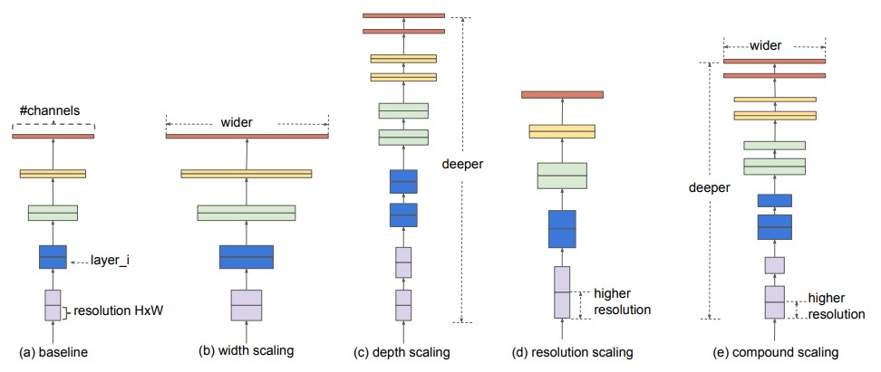
This is the central insight of EfficientNet. A convolutional neural network (CNN) has three “dimensions” you can scale:

• Depth: how many layers deep the network is.
• Width: how many channels (feature maps) each layer has.
• Resolution: the spatial size of the input image.

Before EfficientNet, researchers typically scaled only one of these dimensions at a time. EfficientNet introduced a simple but powerful principle: scale all three together, in a coordinated way, using a single compound coefficient. The result was a family of models that matched or outperformed much larger networks at a fraction of the compute cost.

1. Why Scaling Matters

1.1 The Problem with One-Dimensional Scaling

To understand why compound scaling matters, think about what happens when you scale only one dimension:

• Deeper only: each layer must process images at the same limited resolution with the same number of channels. After a certain depth, accuracy gains plateau because the network lacks the representational capacity at each layer to process richer detail.
• Wider only: more channels per layer give richer representations per stage, but without sufficient depth, the network cannot combine low-level features into high-level concepts.
• Higher resolution only: bigger images carry more detail, but if the network is too small to process that detail, most of it is wasted.

Empirically, each one-dimensional scaling strategy hits diminishing returns quickly. This is not merely a theoretical concern, it was observed consistently in practice before EfficientNet.

1.2 The Compound Scaling Insight

The key observation is that depth, width, and resolution are interdependent. A higher-resolution image benefits from more layers (to capture long-range spatial relationships) and more channels (to represent richer features at each scale). Increasing one without the others leaves capacity on the table.

EfficientNet formalizes this by tying all three dimensions to a single budget parameter $\phi$. Think of $\phi$ as a “volume knob”: turning it up increases depth, width, and resolution together. The exact ratios are fixed by a one-time search on the baseline model.

2. The Math Behind Compound Scaling

2.1 The Scaling Equations

Given a baseline network and a compound coefficient $\phi$, EfficientNet scales the three dimensions as follows:

$$
\text{depth:} \quad d = \alpha^{\phi}
$$

$$
\text{width:} \quad w = \beta^{\phi}
$$

$$
\text{resolution:} \quad r = \gamma^{\phi}
$$

where $\alpha$, $\beta$, and $\gamma$ are fixed constants determined by a small grid search. They are subject to the constraint:

$$
\alpha \cdot \beta^2 \cdot \gamma^2 \approx 2
$$

The intuition: each step in $\phi$ should roughly double the compute budget (FLOPs). The exponents ensure that as you increase $\phi$, the compute scales predictably, allowing you to choose a model size that fits your resource constraints.

In the original paper, the authors found that scaling depth by $\alpha = 1.2$, width by $\beta = 1.1$, and resolution by $\gamma = 1.15$ worked well across a range of compute budgets. This means that for each step in $\phi$, depth increases by 20%, width by 10%, and resolution by 15%, resulting in a predictable doubling of compute.

2.2 Why the Exponents Are What They Are

For a typical convolution layer, FLOPs scale as:

$$
\text{FLOPs} \propto H \cdot W \cdot C_{\text{in}} \cdot C_{\text{out}} \cdot k^2
$$

where $H, W$ are spatial dimensions, $C$ is the number of channels, and $k$ is the kernel size.

Now trace what happens when you apply the three multipliers:

• Scaling depth by $d$ adds more layers linearly, so compute scales as $\propto d$.
• Scaling width by $w$ multiplies both $C_{\text{in}}$ and $C_{\text{out}}$, so compute scales as $\propto w^2$.
• Scaling resolution by $r$ multiplies both $H$ and $W$, so compute scales as $\propto r^2$.

The total compute scales roughly as:

$$
\text{FLOPs}(d, w, r) \approx \text{FLOPs}_0 \cdot d \cdot w^2 \cdot r^2
$$

Substituting the scaling rules:

$$
\text{FLOPs}(\phi) \approx \text{FLOPs}_0 \cdot (\alpha \cdot \beta^2 \cdot \gamma^2)^{\phi} \approx \text{FLOPs}_0 \cdot 2^{\phi}
$$

So each step in $\phi$ doubles the compute budget. This gives a predictable, principled scaling ladder: EfficientNet-B0 ($\phi = 0$), B1 ($\phi = 1$), …, B7 ($\phi = 7$).

3. The EfficientNet-B0 Architecture

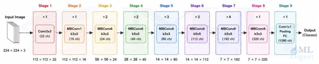
EfficientNet-B0 is the baseline model found through neural architecture search (NAS), optimized under a mobile-level FLOP constraint. It uses two key building blocks.

3.1 MBConv: The Mobile Inverted Bottleneck

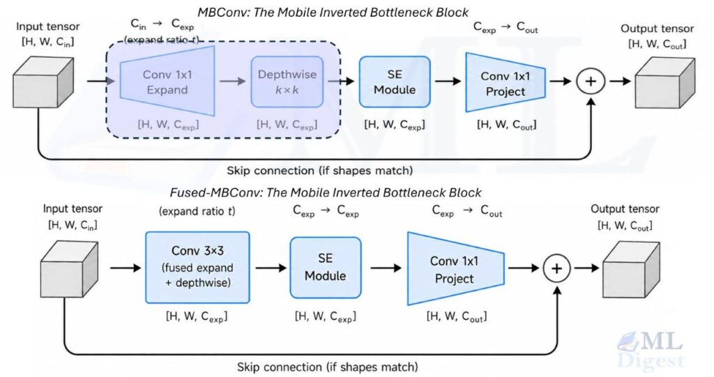
The workhorse of EfficientNet is the MBConv block, popularized by MobileNetV2. The “inverted bottleneck” name comes from the fact that it first expands the number of channels (making the representation richer), performs spatial filtering in that expanded space, and then projects back down to a narrower output.

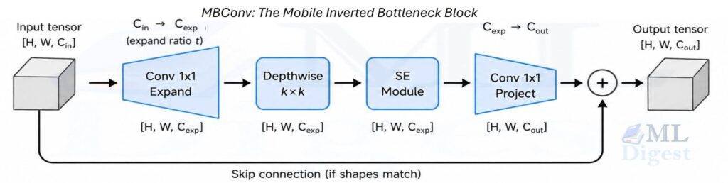
A single MBConv block performs these steps in sequence:

1. 1×1 expansion convolution: scales up channels by an expansion ratio.
2. Depthwise k x k convolution: applies a separate spatial filter per channel (no channel mixing yet). EfficientNet uses kernel sizes of 3 and 5 in different stages.
3. Squeeze-and-Excitation (SE): a lightweight channel-attention gate (described next).
4. 1×1 projection convolution: compresses back to the output channel count.
5. Skip connection: adds the input directly to the output when the shapes match (just like residual connections in ResNet-style networks).

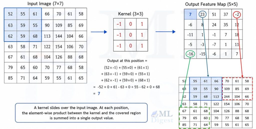
The efficiency gain comes from the depthwise step. A standard convolution mixes all input channels at every spatial location simultaneously. A depthwise convolution filters each channel independently, dramatically reducing the compute:

$$
\text{Standard conv FLOPs:} \quad H \cdot W \cdot C_{\text{in}} \cdot C_{\text{out}} \cdot k^2
$$

$$
\text{Depthwise + pointwise FLOPs:} \quad H \cdot W \cdot C_{\text{in}} \cdot (k^2 + C_{\text{out}})
$$

When $C_{\text{out}}$ is large (as is typical), the savings are significant. For example, with $k=3$ and $C_{\text{out}} = 128$, the full depthwise-plus-pointwise block uses about $(9 + 128) / (9 \cdot 128) \approx 12\%$ of the FLOPs of a standard $3 \times 3$ convolution with the same channel counts.

3.2 Squeeze-and-Excitation (SE)

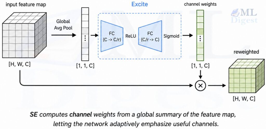
Inside each MBConv block, after the depthwise convolution, there is a small Squeeze-and-Excitation module. SE adds channel-wise attention: the network learns to emphasize which feature channels are most useful for the current image.

The three steps are:

1. Squeeze: global average pooling reduces the feature map from shape $[H, W, C]$ to $[1,1,C]$. This summarizes “what is present” across the entire image.
2. Excite: a two-layer fully connected network (with a bottleneck, reducing $C$ to $C/r$ and back to $C$) takes this summary and produces a weight for each channel, squashed through a sigmoid to land in $(0, 1)$.
3. Scale: each channel in the original feature map is multiplied by its learned weight.

Intuitively, SE lets the network say, “for this image, the ‘texture’ channels matter a lot and the ‘edge’ channels matter less, so reweight accordingly.”

3.3 Swish Activation

EfficientNet replaces the standard ReLU with the Swish activation function (also known as SiLU):

$$
\text{Swish}(x) = x \cdot \sigma(x) = \frac{x}{1 + e^{-x}}
$$

Unlike ReLU, Swish is smooth everywhere and non-monotonic: it allows small negative values near zero to pass through, which empirically helps optimization in deep networks. In PyTorch, this is torch.nn.SiLU().

3.4 Stochastic Depth

EfficientNet also uses stochastic depth during training. At each training step, each residual block is either kept (with probability $p$) or its residual branch is dropped (the skip connection still passes through). This is analogous to Dropout but applied at the block level, making it one instance of the broader family of regularization techniques in neural networks.

The practical effect: the network implicitly trains a large ensemble of sub-networks of varying depths, improving generalization without increasing inference cost.

4. EfficientNet-B0 Through B7

B0 is the baseline. B1 through B7 apply increasing values of $\phi$, which translates into higher input resolution, more channels, and more layers. The progression is smooth because the scaling ratios $(\alpha, \beta, \gamma)$ are fixed.

As a rough practical guide:

• B0 and B1: strong accuracy with very low compute. Good starting points for resource-constrained settings.
• B2 and B3: a common sweet spot for many applied tasks, offering meaningfully better accuracy for a moderate compute increase.
• B4 and B5: for settings where accuracy is the primary concern and compute is not tightly constrained.
• B6 and B7: the heaviest variants. Useful when you want to push accuracy to the limit and have the GPU memory to support large input resolutions (up to 600×600).

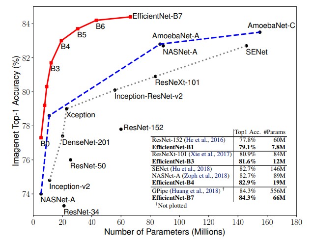
Note that the scaling trend is monotonic, but not an exact per-step doubling once channel counts, depths, and input resolutions are rounded to practical values. In the original family, B0 has about 5.3M parameters and 0.39B FLOPs, B1 has 7.8M parameters and 0.70B FLOPs, B2 has 9.2M parameters and 1.0B FLOPs, and so on, with each step roughly doubling the compute. The accuracy on ImageNet also improves with each step, but with diminishing returns: B0 achieves 77.1% top-1 accuracy, while B7 reaches 84.4%, but the jump from B0 to B1 is much larger than from B6 to B7.

5. EfficientNetV2: Faster Training, Better Efficiency

EfficientNetV2 (Tan and Le, 2021) revisits the design with a focus on training speed in addition to inference efficiency.

5.1 Fused-MBConv

In the early stages of EfficientNet-B0, the input feature maps are large spatially but have few channels. In this regime, the depthwise-then-pointwise decomposition is not always faster in practice on modern hardware because the small depthwise operations are memory-bandwidth-bound.

EfficientNetV2 replaces the depthwise + pointwise steps in early stages with a single regular 3×3 convolution, called Fused-MBConv. This trades a small increase in FLOPs for better hardware utilization and measurably faster wall-clock training.

5.2 Progressive Learning

EfficientNetV2 also trains with a progressive learning strategy: early in training, smaller images with weaker regularization are used. As training progresses, image size increases and regularization (mixup, random augmentation) intensifies. This speeds up early training epochs while still exposing the model to full-resolution images later, where fine-grained features matter.

5.3 When to Choose V2

If your framework supports EfficientNetV2 (both timm and modern torchvision do), it is generally a better default than the original EfficientNet for new projects. The training is faster, the parameter efficiency is better, and the accuracy at comparable sizes is improved.

6. Transfer Learning Workflow

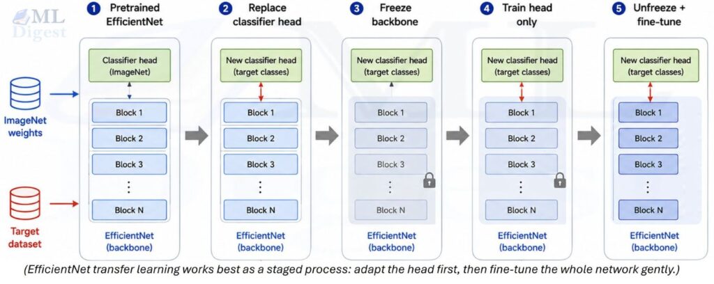
For most practitioners, EfficientNet is not trained from scratch. It is used as a pretrained backbone, fine-tuned on a target dataset. Here is a practical transfer learning workflow.

6.1 The Standard Protocol

1. Load pretrained weights from ImageNet.
2. Replace the final classifier head with a new nn.Linear(in_features, num_classes).
3. Freeze all backbone parameters (except the new head) and train for a few epochs to warm up the new head.
4. Unfreeze the full network and fine-tune end-to-end with a small learning rate (typically $10^{-4}$ or lower).

This two-phase approach prevents the randomly initialized head from destroying pretrained features during early training.

6.2 Practical Tips

• Always use the preprocessing that matches the pretrained weights. For torchvision, prefer weights.transforms() rather than hard-coding resize, crop, interpolation, mean, and std. Many ImageNet checkpoints do use mean [0.485, 0.456, 0.406] and std [0.229, 0.224, 0.225], but the resize and interpolation settings can still differ across variants.
• Match the input resolution. B0 expects 224×224 by default. Using a different resolution requires adjusting the model or accepting that the pretrained spatial priors do not exactly align.
• For small datasets (a few thousand examples), heavier augmentation (random crop, color jitter, RandAugment, random erasing) matters more than model size. Consider B0 or B1 with strong augmentation over B5 with weak augmentation.
• When fine-tuning, use a learning rate schedule that decays over the fine-tuning phase (cosine annealing or step decay work well). If you want to compare common decay policies, this learning rate schedule guide is a useful companion.

7. Code Examples

pip install timm torch torchvision

import torch
import timm

def main():
    # Load pretrained EfficientNet-B0 (downloads weights on first run)
    model = timm.create_model("efficientnet_b0", pretrained=True)
    model.eval()

    # Dummy batch: 1 RGB image at 224x224
    x = torch.randn(1, 3, 224, 224)

    with torch.inference_mode():
        logits = model(x)
        probs = logits.softmax(dim=-1)

    print("Output logits shape:", logits.shape)   # (1, 1000) for ImageNet
    print("Top-5 prob sum:", probs.topk(5, dim=-1).values.sum().item())

if __name__ == "__main__":
    main()
# Expect output:
#     Output logits shape: torch.Size([1, 1000])
#     Top-5 prob sum: 0.017089735716581345

import torch
import timm

def main():
    # Load pretrained EfficientNet-B0 (downloads weights on first run)
    model = timm.create_model("efficientnet_b0", pretrained=True)
    model.eval()

    # Dummy batch: 1 RGB image at 224x224
    x = torch.randn(1, 3, 224, 224)

    with torch.inference_mode():
        logits = model(x)
        probs = logits.softmax(dim=-1)

    print("Output logits shape:", logits.shape)   # (1, 1000) for ImageNet
    print("Top-5 prob sum:", probs.topk(5, dim=-1).values.sum().item())

if __name__ == "__main__":
    main()
# Expect output:
#     Output logits shape: torch.Size([1, 1000])
#     Top-5 prob sum: 0.017089735716581345

import torch
import torch.nn as nn
import timm
from torch.utils.data import DataLoader

def make_model(num_classes: int, model_name: str = "efficientnet_b0") -> nn.Module:
    """
    Load a pretrained EfficientNet and replace its classification head.
    timm exposes the classifier as model.classifier for EfficientNet variants.
    """
    model = timm.create_model(model_name, pretrained=True)
    in_features = model.classifier.in_features
    model.classifier = nn.Linear(in_features, num_classes)
    return model


def freeze_backbone(model: nn.Module) -> None:
    """Freeze all parameters except the new classifier head."""
    for name, param in model.named_parameters():
        if not name.startswith("classifier"):
            param.requires_grad = False


def unfreeze_all(model: nn.Module) -> None:
    """Unfreeze all parameters for end-to-end fine-tuning."""
    for param in model.parameters():
        param.requires_grad = True


def count_params(model: nn.Module) -> tuple[int, int]:
    trainable = sum(p.numel() for p in model.parameters() if p.requires_grad)
    total = sum(p.numel() for p in model.parameters())
    return trainable, total


if __name__ == "__main__":
    NUM_CLASSES = 10

    model = make_model(num_classes=NUM_CLASSES)
    freeze_backbone(model)

    trainable, total = count_params(model)
    print(f"Phase 1 (head only): {trainable:,} trainable / {total:,} total parameters")

    # --- Phase 1: train only the head ---
    optimizer = torch.optim.AdamW(
        filter(lambda p: p.requires_grad, model.parameters()),
        lr=1e-3
    )

    # --- After a few epochs, unfreeze for full fine-tuning ---
    unfreeze_all(model)
    trainable, _ = count_params(model)
    print(f"Phase 2 (full model): {trainable:,} trainable parameters")

    optimizer = torch.optim.AdamW(model.parameters(), lr=1e-4)
# Expect output:
#     Phase 1 (head only): 12,810 trainable / 4,020,358 total parameters
#     Phase 2 (full model): 4,020,358 trainable parameters

import torch
import torch.nn as nn
import timm
from torch.utils.data import DataLoader

def make_model(num_classes: int, model_name: str = "efficientnet_b0") -> nn.Module:
    """
    Load a pretrained EfficientNet and replace its classification head.
    timm exposes the classifier as model.classifier for EfficientNet variants.
    """
    model = timm.create_model(model_name, pretrained=True)
    in_features = model.classifier.in_features
    model.classifier = nn.Linear(in_features, num_classes)
    return model


def freeze_backbone(model: nn.Module) -> None:
    """Freeze all parameters except the new classifier head."""
    for name, param in model.named_parameters():
        if not name.startswith("classifier"):
            param.requires_grad = False


def unfreeze_all(model: nn.Module) -> None:
    """Unfreeze all parameters for end-to-end fine-tuning."""
    for param in model.parameters():
        param.requires_grad = True


def count_params(model: nn.Module) -> tuple[int, int]:
    trainable = sum(p.numel() for p in model.parameters() if p.requires_grad)
    total = sum(p.numel() for p in model.parameters())
    return trainable, total


if __name__ == "__main__":
    NUM_CLASSES = 10

    model = make_model(num_classes=NUM_CLASSES)
    freeze_backbone(model)

    trainable, total = count_params(model)
    print(f"Phase 1 (head only): {trainable:,} trainable / {total:,} total parameters")

    # --- Phase 1: train only the head ---
    optimizer = torch.optim.AdamW(
        filter(lambda p: p.requires_grad, model.parameters()),
        lr=1e-3
    )

    # --- After a few epochs, unfreeze for full fine-tuning ---
    unfreeze_all(model)
    trainable, _ = count_params(model)
    print(f"Phase 2 (full model): {trainable:,} trainable parameters")

    optimizer = torch.optim.AdamW(model.parameters(), lr=1e-4)
# Expect output:
#     Phase 1 (head only): 12,810 trainable / 4,020,358 total parameters
#     Phase 2 (full model): 4,020,358 trainable parameters

import torch
from torchvision.models import efficientnet_b0, EfficientNet_B0_Weights

# Load with ImageNet weights using the recommended enum-based API
model = efficientnet_b0(weights=EfficientNet_B0_Weights.IMAGENET1K_V1)
model.eval()

x = torch.randn(1, 3, 224, 224)
with torch.inference_mode():
    logits = model(x)

print("Output shape:", logits.shape)  # torch.Size([1, 1000])

import torch
from torchvision.models import efficientnet_b0, EfficientNet_B0_Weights

# Load with ImageNet weights using the recommended enum-based API
model = efficientnet_b0(weights=EfficientNet_B0_Weights.IMAGENET1K_V1)
model.eval()

x = torch.randn(1, 3, 224, 224)
with torch.inference_mode():
    logits = model(x)

print("Output shape:", logits.shape)  # torch.Size([1, 1000])

import torch.nn as nn
from torchvision.models import efficientnet_b0, EfficientNet_B0_Weights

model = efficientnet_b0(weights=EfficientNet_B0_Weights.IMAGENET1K_V1)
in_features = model.classifier[1].in_features
model.classifier[1] = nn.Linear(in_features, out_features=10)

import torch.nn as nn
from torchvision.models import efficientnet_b0, EfficientNet_B0_Weights

model = efficientnet_b0(weights=EfficientNet_B0_Weights.IMAGENET1K_V1)
in_features = model.classifier[1].in_features
model.classifier[1] = nn.Linear(in_features, out_features=10)

8. Choosing the Right Variant

Here is a concise decision guide:

By compute budget:

• Tight latency / edge deployment: start with efficientnet_b0 or efficientnet_b1.
• Balanced (most applications): efficientnet_b3 or efficientnet_b4.
• Accuracy-first: efficientnet_b5 through efficientnet_b7, or any EfficientNetV2 variant.

By framework preference:

• Recommended for most new projects: timm with tf_efficientnetv2_s or tf_efficientnetv2_m.
• Standard torchvision install: efficientnet_b0 through efficientnet_b7.

If transfer learning accuracy is insufficient:

1. First, check data quality and augmentation. Strong augmentation (RandAugment, Mixup, CutMix) often matters more than model size.
2. Unfreeze earlier layers and fine-tune longer with a smaller learning rate.
3. Increase input resolution moderately (for example, 224 to 256 or 288).
4. Move up one model size (for example, B2 to B3).
5. Switch to EfficientNetV2 for a better accuracy/cost trade-off.

When EfficientNet may not be the best choice:

• On some GPU architectures, depthwise convolutions are less cache-efficient than standard convolutions, and a model like ConvNeXt may run faster at comparable accuracy.
• For very large datasets (hundreds of millions of images), Vision Transformers (like DETR) and hybrid architectures often pull ahead. EfficientNet was designed with the ImageNet-scale regime in mind.

Summary

EfficientNet makes a single elegant argument: if you want more accurate CNNs, do not scale one dimension arbitrarily. Scale all three dimensions (depth, width, and resolution) in proportion to your compute budget, using the compound coefficient $\phi$.

The practical toolkit is:

• MBConv with Squeeze-and-Excitation: a mobile-friendly building block that combines cheap depthwise convolutions with learned channel attention.
• Swish activation: a smooth, trainable-friendly alternative to ReLU.
• Stochastic depth: block-level Dropout for better generalization.
• Compound scaling: a one-parameter family of models from B0 to B7 that increases depth, width, and resolution together so compute rises in a controlled way.

EfficientNetV2 extends this by swapping in Fused-MBConv for early stages and using progressive learning with adaptive regularization, improving training speed and parameter efficiency.

For most applied computer vision tasks, starting with a pretrained EfficientNet-B0 or EfficientNetV2-S and fine-tuning it is usually a much stronger baseline than training a small custom CNN from scratch. The pretrained weights encode general visual features learned from millions of images, and the compound scaling design helps avoid wasting compute on imbalanced capacity.

S L Happy

Machine Learning Engineer at HP | Website |  + postsBio ⮌

Happy is a seasoned ML professional with over 15 years of experience. His expertise spans various domains, including Computer Vision, Natural Language Processing (NLP), and Time Series analysis. He holds a PhD in Machine Learning from IIT Kharagpur and has furthered his research with postdoctoral experience at INRIA-Sophia Antipolis, France. Happy has a proven track record of delivering impactful ML solutions to clients.

• S L Happy

  Detection Transformers (DETR) Made Easy: End-to-End Object Detection with Transformers
• S L Happy

  BM25 Made Easy: Visualizing the Core of Modern Search
• S L Happy

  What Are Knowledge Graph-Based RAG Systems? Complete Beginner’s Guide
• S L Happy

  Evaluation Metrics in Machine Learning: A Practical Field Guide

Silpa

Website |  + postsBio ⮌

Silpa brings 5 years of experience in working on diverse ML projects, specializing in designing end-to-end ML systems tailored for real-time applications. Her background in statistics (Bachelor of Technology) provides a strong foundation for her work in the field. Silpa is also the driving force behind the development of the content you find on this site.

• Silpa

  Detection Transformers (DETR) Made Easy: End-to-End Object Detection with Transformers
• Silpa

  BM25 Made Easy: Visualizing the Core of Modern Search
• Silpa

  What Are Knowledge Graph-Based RAG Systems? Complete Beginner’s Guide
• Silpa

  Evaluation Metrics in Machine Learning: A Practical Field Guide