Imagine you hired the world’s most brilliant employee. They can write code, summarize legal contracts, generate marketing copy, and answer customer questions, all at superhuman speed. There is just one problem: they charge you for every single word they read or write, they need a dedicated server farm to think, and training them from scratch costs hundreds of millions of dollars. That is the reality of working with Large Language Models today.
LLMs are transformative, but they are expensive in three distinct ways: the cost to train them, the cost to serve them at inference time, and the infrastructure cost that underlies everything. Whether you are a researcher squeezing experiments into a tight GPU budget or an engineer keeping your production API bill under control, understanding where the money goes, and how to reduce it, is one of the most practically useful skills in the modern ML toolkit.
This guide walks you through all three cost dimensions, the mathematical intuition behind the savings, and concrete code examples you can use right away.
1. Where Does the Money Actually Go?
Before we start cutting costs, let us understand what we are paying for. LLM costs can be decomposed into three broad buckets.
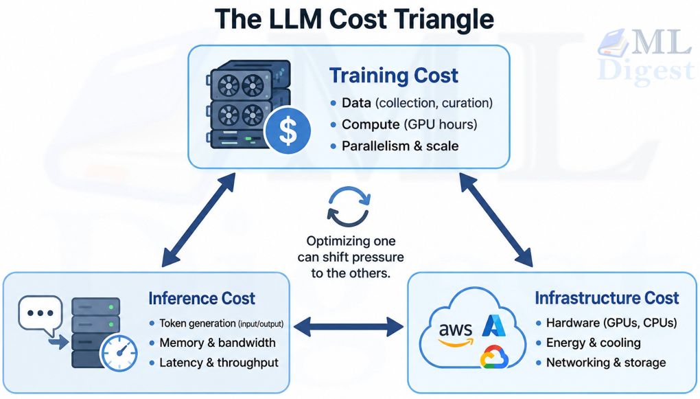
Training cost is the one-time (or periodic) expense of running gradient descent over billions of tokens. A single training run for a frontier model can cost tens of millions of dollars in compute alone. For most practitioners, this manifests as fine-tuning costs on proprietary or open-source base models.
Inference cost is the ongoing, per-request expense of generating tokens. In a high-traffic production system, inference can quickly dwarf training cost. OpenAI, Anthropic, and Google all charge per input and output token, and those numbers add up fast.
Infrastructure cost is the foundational layer: the hardware, cloud instances, networking, storage, and engineering time required to keep everything running. It affects both training and inference but has its own optimization levers.
2. Training Cost Reduction
Training is where models are born, but it can also be where budgets go to die. Here is how to train smarter.
2.1 Mixed Precision Training
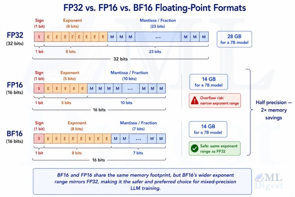
The simplest, highest-return optimization for training is switching from 32-bit floating point (FP32) to 16-bit (FP16 or BF16). This cuts memory usage nearly in half and, on modern GPUs, roughly doubles throughput because tensor cores operate in 16-bit.
The math is straightforward. A model with $N$ parameters stored in FP32 requires:
$$\text{Memory}_{\text{FP32}} = 4N \text{ bytes}$$
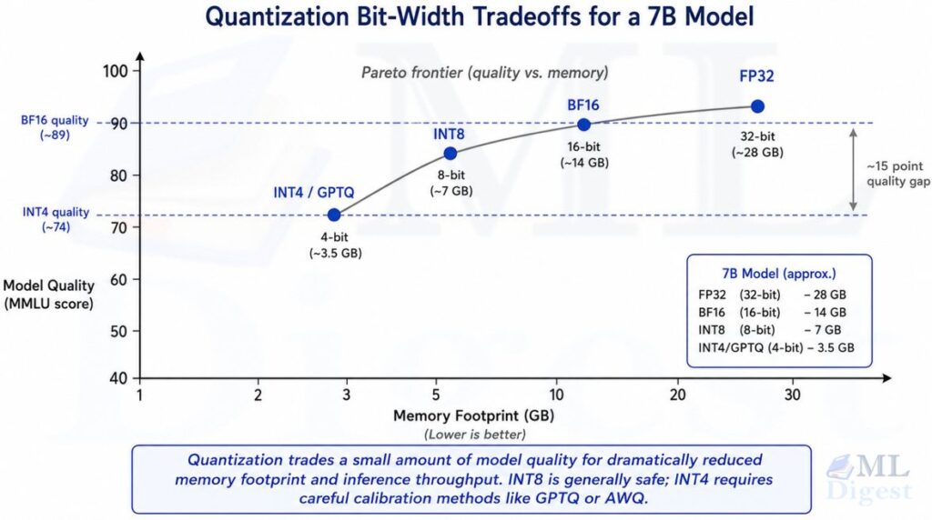
Switching to BF16 halves this to $2N$ bytes per parameter. For a 7B parameter model, that is roughly 14 GB instead of 28 GB, often the difference between fitting on one GPU or needing two.
BF16 is generally preferred over FP16 for training because it has the same exponent range as FP32 (8 bits vs. FP16’s 5 bits), meaning it handles the large gradient magnitudes common in training without overflow.
Pseudo-code to train models with different precision
import torch
from torch.cuda.amp import autocast, GradScaler

model = MyTransformerModel().cuda()
optimizer = torch.optim.AdamW(model.parameters(), lr=3e-4)
scaler = GradScaler()  # handles FP16 gradient scaling (for BF16, you can skip this)

for batch in dataloader:
    optimizer.zero_grad()

    # Forward pass in FP16
    with autocast(dtype=torch.float16):
        outputs = model(batch["input_ids"])
        loss = outputs.loss

    # Backward pass: scaler prevents underflow in FP16 gradients
    scaler.scale(loss).backward()
    scaler.step(optimizer)
scaler.update()2.2 Gradient Checkpointing
During a standard forward pass, PyTorch stores all intermediate activations so they are available during backpropagation. For a deep transformer, activation storage can consume several gigabytes of memory across the training stack. Gradient checkpointing trades computation for memory: it discards intermediate activations during the forward pass and recomputes them on the fly during the backward pass.
The tradeoff is roughly 20-40% more computation in exchange for a large reduction in activation memory across the network, often enabling a much larger batch size, which can actually improve GPU utilization and net throughput.
from torch.utils.checkpoint import checkpoint_sequential

# Wrap your transformer layers with gradient checkpointing
# PyTorch recomputes activations during backward instead of caching them
output = checkpoint_sequential(model.layers, segments=4, input=hidden_states)With Hugging Face Transformers, enabling it is a single line:
model.gradient_checkpointing_enable()2.3 Parameter-Efficient Fine-Tuning (PEFT)
This is the single biggest lever for reducing fine-tuning cost. Parameter-efficient fine-tuning (PEFT) methods freeze most of the base model and only train a small number of new or modified parameters. The Hugging Face PEFT library implements the most widely used methods and integrates seamlessly with Transformers.
LoRA: Low-Rank Adaptation
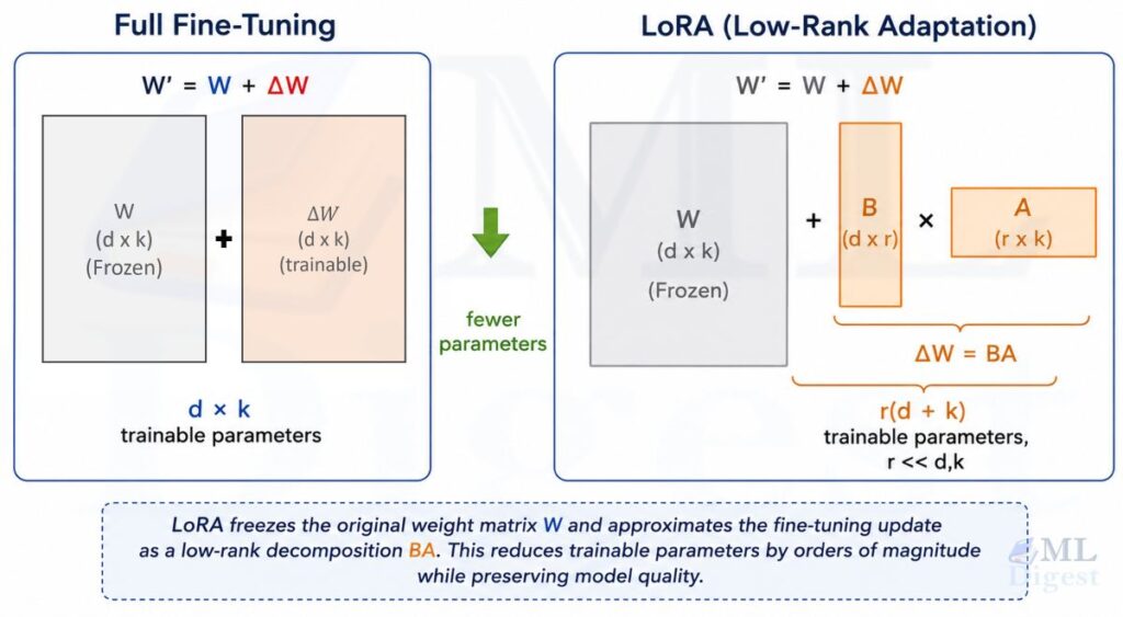
LoRA is the most widely adopted PEFT method. The key insight is that the update to a weight matrix $W \in \mathbb{R}^{d \times k}$ during fine-tuning tends to have low intrinsic rank. LoRA approximates this update as the product of two smaller matrices:
$$W’ = W + \Delta W = W + BA$$
where $B \in \mathbb{R}^{d \times r}$ and $A \in \mathbb{R}^{r \times k}$, and $r \ll \min(d, k)$ is the rank hyperparameter. Instead of updating $d \times k$ parameters, LoRA only trains $r(d + k)$ parameters.
For a typical attention projection layer with $d = k = 4096$ and $r = 8$:
- Full fine-tuning: $4096 \times 4096 = 16{,}777{,}216$ parameters
- LoRA: $8 \times (4096 + 4096) = 65{,}536$ parameters, a reduction of 256x
QLoRA: Quantize First, Then LoRA
QLoRA (Dettmers et al., 2023) pushes this further by first quantizing the frozen base model to 4-bit NormalFloat (NF4) and then applying LoRA adapters. It enables fine-tuning a 65B parameter model on a single 48 GB GPU, a task that would otherwise require 160+ GB of GPU memory.
2.4 Data Efficiency
The most overlooked training cost driver is data quality. Training on more tokens is not always better if the data is noisy or redundant. Several strategies can reduce the effective compute required:
Data deduplication removes near-duplicate documents that would otherwise be seen multiple times, wasting gradient steps. The Deduplication paper showed that deduplication not only reduces training cost but also improves downstream performance by reducing memorization.
Curriculum learning presents easier examples first and harder ones later, mimicking how humans learn. This can reduce the total number of training steps needed to reach a target loss.
Dataset pruning uses techniques like DSIR (Data Selection via Importance Resampling) to select the most informative training examples for a given target task, allowing you to train on a smaller but more effective dataset.
Meta-learning takes a different angle entirely. Instead of choosing better data, meta-learning optimizes for rapid adaptation across a distribution of tasks so that the learned initialization can be adapted to a new task with only a few gradient steps and therefore very little task-specific data. The most well-known formulation is MAML (Model-Agnostic Meta-Learning, Finn et al. 2017), where the objective is to find parameters $\theta$ such that a small number of gradient steps on any new task $\mathcal{T}_i$ produces a high-performing model:
$$\theta^* = \arg\min_\theta \sum_{\mathcal{T}_i \sim p(\mathcal{T})} \mathcal{L}_{\mathcal{T}_i}\left(\theta – \alpha \nabla_\theta \mathcal{L}_{\mathcal{T}_i}(\theta)\right)$$
In the LLM context, the intuition is related but the training objective is usually different. Modern instruction tuning and multitask pre-training are not typically described as MAML-style meta-learning; instead, they broaden the task distribution the model sees so it transfers better in zero-shot and few-shot settings. That is why instruction-tuned models like Flan-T5 and Llama-3-Instruct often need far fewer labeled examples for downstream adaptation than training from scratch.
2.5 Efficient Distributed Training
For large-scale training, how you distribute computation across GPUs significantly affects cost. The three main parallelism strategies are:
Data parallelism (DP): Each GPU holds a full model copy and processes a different batch. Gradients are synchronized via all-reduce. Efficient but memory-constrained to one model copy per GPU.
Tensor parallelism (TP): Individual weight matrices are split across GPUs. Each GPU holds a slice of each layer. Requires high-bandwidth interconnects (NVLink) to be efficient.
Pipeline parallelism (PP): Different layers are assigned to different GPUs. The model is a pipeline of stages. Introduces “pipeline bubbles” (idle time) that must be minimized with micro-batching.
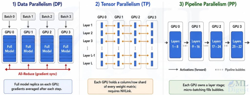
DeepSpeed ZeRO (Zero Redundancy Optimizer) is the practical workaround for most teams: it shards optimizer states, gradients, and parameters across data-parallel ranks, eliminating redundancy without requiring model-parallel refactoring.
2.6 Sparse Training and Mixture of Experts
A dense transformer processes every token through every parameter in every layer. That is thorough, but also expensive. Sparse training challenges this assumption: what if only a subset of the model’s capacity needed to activate for any given input?
The modern realization of this idea is Mixture of Experts (MoE). In an MoE layer, the standard feed-forward block is replaced with $E$ parallel expert networks and a lightweight router. For each token, the router selects the top $k$ experts (typically $k = 2$) and only those experts compute on that token. The output is a weighted combination of the selected experts’ outputs:
$$\text{MoE}(x) = \sum_{i=1}^{k} g_i(x) \cdot E_i(x), \quad \text{where } g_i = \text{softmax}(\text{router}(x))_i$$
The critical insight for cost: with 8 experts and $k = 2$, each token activates only 25% of the total MoE parameters. You get a model with the total parameter count (and thus representational capacity) of a large model, but the per-token compute cost of a much smaller one. Mixtral-8x7B (Jiang et al., 2024) has 47B total parameters but only 13B active parameters per token, matching or exceeding LLaMA 2-70B quality at a fraction of the inference cost.
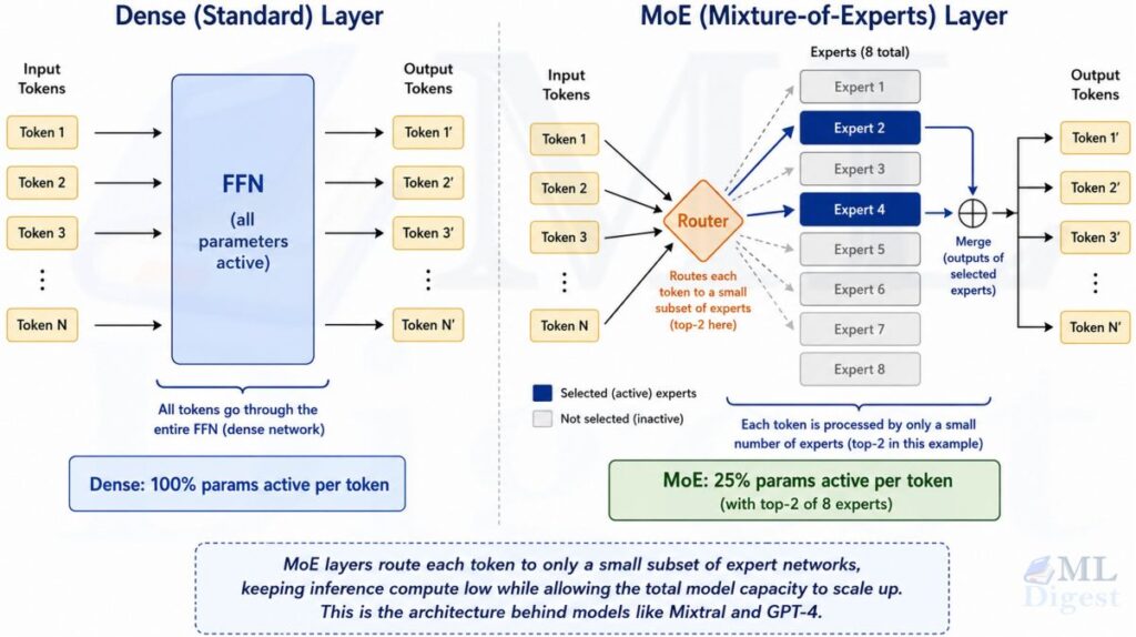
Load balancing is an important practical concern in MoE training: if the router always selects the same few experts, capacity is wasted. An auxiliary load-balancing loss penalizes uneven expert utilization and is added to the training objective alongside the primary language modeling loss.
3. Inference Cost Reduction
Inference is where most production costs live. Every user query triggers a forward pass, and with millions of users, even small per-token savings compound dramatically.
3.1 Quantization at Inference Time
Quantization reduces the numerical precision of model weights (and sometimes activations) to use fewer bits per value. At inference, this means smaller memory footprint, faster memory bandwidth utilization, and often access to specialized integer arithmetic on modern hardware.
The general formulation maps a floating-point value $x$ to a quantized integer $x_q$:
$$x_q = \text{round}\left(\frac{x}{s}\right) + z$$
where $s$ is a scale factor and $z$ is a zero-point. During dequantization:
$$\hat{x} = s(x_q – z)$$
The error introduced, $\hat{x} – x$, is the quantization error, which accumulates across layers and affects output quality.
INT8 post-training quantization (PTQ) is usually the safest starting point: it halves weight memory and often improves throughput, while model-quality impact is frequently small but still task- and model-dependent. The bitsandbytes library provides a convenient interface for this, integrated directly into Hugging Face Transformers:
from transformers import AutoModelForCausalLM, BitsAndBytesConfig

# INT8 inference via bitsandbytes
bnb_int8_config = BitsAndBytesConfig(load_in_8bit=True)

model = AutoModelForCausalLM.from_pretrained(
    "mistralai/Mistral-7B-v0.1",
    quantization_config=bnb_int8_config,
    device_map="auto",
)GPTQ (Post-Training Quantization for GPT models, Frantar et al. 2022) applies a layer-wise second-order optimization to minimize quantization error, enabling aggressive 3-4 bit quantization with much better quality preservation than naive rounding.
AWQ (Activation-aware Weight Quantization, Lin et al. 2023) observes that not all weights are equally important: weights corresponding to large activation channels should be preserved more carefully. AWQ scales the “salient” weights before quantizing, often outperforming GPTQ at the same bit-width.
All three methods above are post-training techniques. Quantization-aware training (QAT) is an alternative that simulates low-precision arithmetic during fine-tuning itself, often recovering accuracy lost by aggressive PTQ at a modest additional training cost.
3.2 Knowledge Distillation
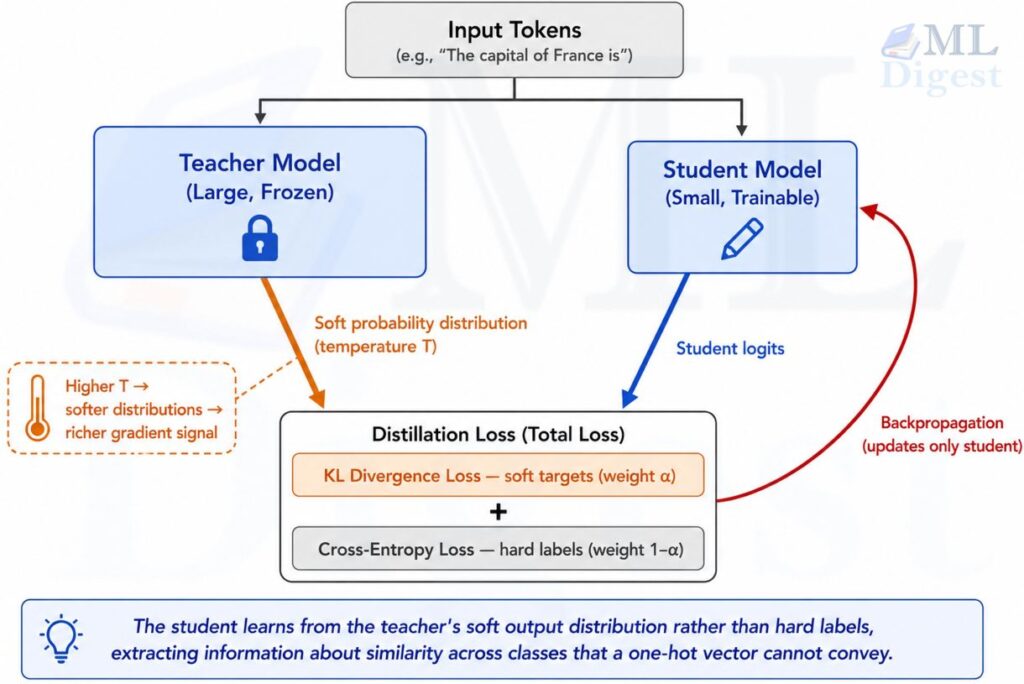
Knowledge distillation, introduced by Hinton et al. (2015), trains a smaller “student” model to mimic the output distribution of a larger “teacher” model. Instead of training on hard labels (one-hot vectors), the student is trained on the teacher’s soft probability distribution, which carries richer information about inter-class similarities.
The distillation loss combines a standard cross-entropy term with a KL-divergence term between student and teacher logits:
$$\mathcal{L}_{\text{distill}} = (1 – \alpha) \mathcal{L}_{\text{CE}}(y, p_s) + \alpha \cdot T^2 \cdot \text{KL}\left(\sigma\left(\frac{z_t}{T}\right) \Bigg| \sigma\left(\frac{z_s}{T}\right)\right)$$
where $z_t$ and $z_s$ are teacher and student logits, $T$ is the temperature (higher $T$ produces softer distributions), and $\alpha$ balances the two loss terms.
Notable distillation successes include DistilBERT (60% faster, 40% smaller, retains 97% of BERT’s performance) and Llama-3.2 small models that were distilled from their larger Llama 3.1 siblings.
Code to perform LLM knowledge distillation
import torch
import torch.nn.functional as F

def distillation_loss(student_logits, teacher_logits, true_labels,
                      temperature=4.0, alpha=0.7):
    """
    Compute the combined distillation + cross-entropy loss.

    Args:
        student_logits: raw logits from the student model
        teacher_logits: raw logits from the frozen teacher model
        true_labels: ground truth token indices
        temperature: softens probability distributions for richer signal
        alpha: weight for the distillation vs. CE loss
    """
    # Soft targets from teacher at temperature T
    soft_teacher = F.softmax(teacher_logits / temperature, dim=-1)
    soft_student = F.log_softmax(student_logits / temperature, dim=-1)

    # KL divergence loss (multiply by T^2 to compensate for gradient scaling)
    kl_loss = F.kl_div(soft_student, soft_teacher, reduction="batchmean") * (temperature ** 2)

    # Standard cross-entropy on hard labels
    ce_loss = F.cross_entropy(student_logits, true_labels)

return alpha * kl_loss + (1 - alpha) * ce_loss3.3 Speculative Decoding
Autoregressive generation is inherently sequential: you cannot generate token $t+1$ until you have token $t$. This serialization bottleneck means that even with a powerful GPU, the model often sits idle waiting for memory bandwidth. Speculative decoding (Leviathan et al., 2022) cleverly exploits this.
The idea: use a small, fast “draft” model to speculatively generate $k$ candidate tokens, then use the large “verifier” model to check all $k$ tokens in a single parallel forward pass (since the verifier can process all $k$ positions simultaneously). If the draft tokens match the verifier’s distribution, you accept them all; otherwise, you fall back.
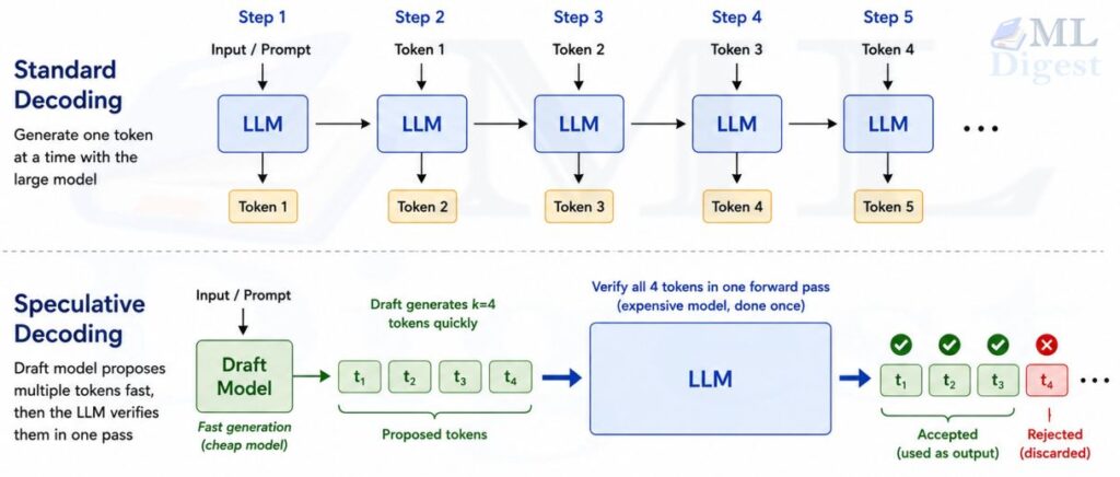
The realized speedup depends on the draft model’s quality, the acceptance rate, the speculation length, and system overhead. In practice, the original paper reports roughly 2x-3x acceleration on T5-XXL, and production gains are strongest when the target model is memory-bandwidth-bound and the draft model is well matched.
Hugging Face transformers supports this natively:
from transformers import AutoModelForCausalLM, AutoTokenizer

# Load large verifier model and small draft model
verifier = AutoModelForCausalLM.from_pretrained("meta-llama/Meta-Llama-3-70B")
draft = AutoModelForCausalLM.from_pretrained("meta-llama/Meta-Llama-3-8B")

tokenizer = AutoTokenizer.from_pretrained("meta-llama/Meta-Llama-3-70B")
inputs = tokenizer("The key insight of transformers is", return_tensors="pt")

# assistant_model triggers speculative decoding automatically
outputs = verifier.generate(
    **inputs,
    assistant_model=draft,  # draft model proposes tokens
    max_new_tokens=200,
)3.4 KV Cache Optimization
During autoregressive generation, the attention mechanism must compute keys and values for all past tokens at every step. To avoid recomputation, these are cached in a KV cache. The problem: the KV cache grows linearly with sequence length, and for long contexts it can consume more memory than the model weights themselves.
The KV cache memory for a transformer with $L$ layers, $H$ KV heads of dimension $d_h$, and sequence length $S$ (in bytes for BF16) is:
$$\text{KV Cache} = 2 \times L \times H \times d_h \times S \times 2 \text{ bytes}$$
For LLaMA 3-8B ($L = 32$, $H = 8$, $d_h = 128$) at 4096 tokens: $2 \times 32 \times 8 \times 128 \times 4096 \times 2 = 536{,}870{,}912$ bytes $\approx$ 512 MB. At 32K tokens, this grows to 4 GB, consuming a substantial fraction of a 24 GB GPU.
Several techniques address this:
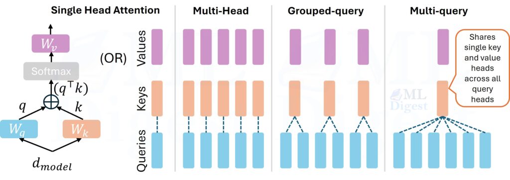
Grouped Query Attention (GQA): Used in LLaMA 2/3, Mistral, and Gemma. Instead of $H$ separate key-value heads (Multi-Head Attention), GQA uses $G < H$ KV heads shared across groups of query heads. With $G = 1$, this becomes Multi-Query Attention (MQA). GQA reduces KV cache by a factor of $H/G$ with minimal quality loss.
Sliding Window Attention: Used in Mistral. Each token only attends to the $W$ most recent tokens rather than all past tokens, capping KV cache at $O(W)$ regardless of sequence length.
Quantized KV Cache: Cache keys and values in INT8 or INT4 instead of BF16, which can cut KV cache memory substantially, though the latency/quality tradeoff depends on context length, backend, and model.
3.5 Efficient Attention: FlashAttention
FlashAttention and its successor FlashAttention-2 do not change the mathematical result of attention, they change where the computation happens. Standard attention materializes the full $N \times N$ attention matrix in GPU HBM (high-bandwidth memory), which requires $O(N^2)$ memory reads and writes. FlashAttention tiles the computation to stay within the much faster SRAM (on-chip cache), drastically reducing HBM access. Critically, this is an IO and memory efficiency optimization: the mathematical output is identical to standard attention up to floating-point rounding.
The speedup is not from doing less work but from doing the same work with fewer expensive memory transfers. In practice, FlashAttention often delivers substantial speedups that become more pronounced at longer sequence lengths, but the exact gain depends heavily on hardware, kernel version, and sequence shape.
Code example
# FlashAttention is built into PyTorch 2.0+ via scaled_dot_product_attention
import torch
import torch.nn.functional as F

# PyTorch automatically dispatches to FlashAttention when available
# (requires CUDA, and input dtype to be float16 or bfloat16)
attn_output = F.scaled_dot_product_attention(
    query, key, value,
    attn_mask=None,
    dropout_p=0.0,
    is_causal=True,  # use causal mask for autoregressive decoding
)3.6 Smart Batching and Continuous Batching
Naively, you might process one request at a time. This leaves the GPU underutilized whenever a request is shorter than the maximum sequence length, because padding fills the rest of the batch with wasted computation.
Dynamic batching groups requests with similar lengths together to minimize padding overhead.
Continuous batching (also called iteration-level scheduling), introduced in Orca, goes further: instead of waiting for all sequences in a batch to finish before starting new ones, it inserts new requests into the batch as soon as a slot becomes available. This dramatically improves GPU utilization for variable-length workloads, which is essentially every real production system.
# vLLM implements continuous batching + PagedAttention out of the box
from vllm import LLM, SamplingParams

llm = LLM(model="mistralai/Mistral-7B-Instruct-v0.2")

# Submit many requests; vLLM schedules them with continuous batching
prompts = [
    "Summarize the French Revolution in two sentences.",
    "Write a Python function to compute Fibonacci numbers.",
    "What is the capital of Morocco?",
]

sampling_params = SamplingParams(temperature=0.7, max_tokens=256)
outputs = llm.generate(prompts, sampling_params)PagedAttention (Kwon et al., 2023), implemented in vLLM, applies virtual-memory-style paging to the KV cache. Instead of pre-allocating a contiguous block of memory for the maximum sequence length (wasting memory on speculative allocation), PagedAttention allocates memory in small fixed-size pages on demand, reducing KV cache fragmentation and enabling much higher throughput.
3.7 Model Pruning
Pruning removes weights (or entire structures) from a trained model that contribute little to its outputs.
Unstructured pruning zeroes out individual weights below a threshold magnitude. It can achieve high sparsity (90%+) but requires sparse matrix libraries to realize actual speedups, since modern GPUs are optimized for dense operations.
Structured pruning removes entire heads, layers, or neurons. The resulting model is a smaller dense model that runs efficiently on standard hardware without special sparse kernels.
Layer dropping is the simplest form of structured pruning: remove entire transformer layers based on their importance score (e.g., cosine similarity between layer input and output). Gromov et al. (2024) showed that the middle layers of LLMs are often the most redundant, and dropping 20-30% of layers from models like LLaMA 2 70B costs only 1-2% on benchmarks while enabling significant inference speedup.
4. Infrastructure Cost Reduction
Even with the best model-level optimizations, infrastructure choices can make or break your unit economics.
4.1 Hardware Selection
Not all GPUs are created equal for LLM workloads. The key metrics to compare are:
Memory bandwidth (GB/s): This is the primary bottleneck for autoregressive decoding, which is memory-bandwidth-bound (you spend most time moving weights from HBM to compute cores, not doing arithmetic). An H100 SXM5 offers 3.35 TB/s vs. the A100’s 2 TB/s.
Compute (TFLOPS): Matters more for training and prefill (prompt processing), which are compute-bound.
Memory capacity (GB): Determines the maximum model size you can fit without offloading.
Price per performance: The A100 and H100 are the workhorses of the industry, but for inference-only workloads, L40S GPUs (48 GB, high memory bandwidth, lower cost than H100) often provide better cost-per-token.
For small-to-medium inference loads, consumer GPUs like the RTX 4090 (24 GB, 1008 GB/s) are remarkably cost-effective for running quantized 7-13B models.
4.2 Spot Instances and Preemptible VMs
Cloud GPU hours at on-demand pricing are expensive. Spot instances (AWS), preemptible VMs (GCP), or interruptible instances (Azure) offer the same hardware at 60-90% discount by allowing the cloud provider to reclaim the instance with short notice.
For training workloads, this requires robust checkpointing: save model state frequently so that a preemption costs only the work since the last checkpoint.
4.3 Model Serving Optimization
The choice of serving framework has an enormous impact on inference throughput and cost. The main options:
vLLM: Best for throughput-optimized serving. Implements PagedAttention and continuous batching. Excellent for batch processing and high-concurrency APIs.
TGI (Text Generation Inference): Hugging Face’s production serving solution. Supports FlashAttention, tensor parallelism, and speculative decoding. Good for single-model deployments with Hugging Face Hub integration.
llama.cpp: CPU-first inference with optional GPU offloading. Exceptional for on-device or edge deployment where GPU memory is very limited. Uses GGUF quantization formats.
TensorRT-LLM: NVIDIA’s graph-compiled serving backend. Highest throughput on NVIDIA hardware by fusing operations and generating hardware-specific code, but requires more setup work.
4.4 Right-Sizing Your Deployment
One of the most common and expensive infrastructure mistakes is over-provisioning. Use auto-scaling to match compute to actual traffic patterns:
For bursty workloads, GPU-backed serverless platforms like Runpod Serverless or Modal can dramatically reduce costs for workloads that are active less than ~30% of the time. By contrast, AWS SageMaker Serverless is designed for CPU-based serverless inference rather than GPU-backed LLM serving. If you are comparing these options more broadly, this connects directly to the tradeoffs in LLM deployment from cloud to edge.
5. Application-Level Cost Reduction
These techniques operate at the application layer, above the model and infrastructure, but can achieve some of the largest practical savings.
5.1 Prompt Compression
Every token you send costs money. Prompt compression techniques reduce the number of tokens in your inputs while preserving the information the model needs. In practice, they work best when paired with disciplined prompt development and management, so repeated instructions and context do not bloat requests in the first place.
LLMLingua uses a small proxy model to score the importance of each token in a long prompt, then drops the least important ones. It achieves 3-20x prompt compression ratios with minimal quality degradation on RAG and summarization tasks.
Summarization-based compression: For RAG applications, instead of retrieving and passing raw document chunks, use a smaller/cheaper model to summarize them first, then pass the summaries to the expensive model.
5.2 Semantic Caching
If 10,000 users ask variations of “What is machine learning?”, should you pay to generate 10,000 answers? Semantic caching stores model responses and returns them for semantically similar future queries, without calling the model at all.
GPTCache is the leading open-source library for this:
from gptcache import cache
from gptcache.adapter import openai

# Initialize cache with semantic similarity matching
cache.init(
    pre_embedding_func=...,       # function to extract cache key from request
    embedding_func=...,           # embedding model for semantic similarity
    data_manager=...,             # storage backend (SQLite, Redis, Milvus, etc.)
    similarity_evaluation=...,    # how to compare cached vs. new query
)

# Now use the drop-in OpenAI replacement; cache is transparent
response = openai.ChatCompletion.create(
    model="gpt-4o",
    messages=[{"role": "user", "content": "What is machine learning?"}],
)On production workloads with high query overlap, semantic caching can reduce API calls by 20-60%.
5.3 LLM Routing: Use the Cheapest Model That Can Do the Job
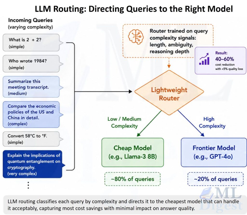
Not every query needs the latest reasoning model. A simple FAQ lookup can be handled by a small, cheap model. A complex multi-step reasoning task genuinely needs a frontier model. LLM routing classifies incoming queries and directs them to the most cost-effective model capable of handling them.
The growing ecosystem of small language models (SLMs) makes this routing strategy increasingly practical, as capable small models are now available at a fraction of the cost of frontier models. RouteLLM trains a lightweight router that predicts whether a query needs a strong model or can be handled by a cheaper one. In their experiments, routing between GPT-4o and Llama-3 70B reduced costs by 40-60% with less than 5% quality degradation on real-world query distributions.
import routellm

# Initialize router (trained to predict strong vs. weak model need)
client = routellm.Controller(
    routers=["mf"],           # matrix factorization-based router
    strong_model="gpt-4o",
    weak_model="gpt-4o-mini",
)

# Router automatically picks the cheaper model when it can
response = client.chat.completions.create(
    model="router-mf-0.11593",  # threshold parameter: lower = more conservative routing
    messages=[{"role": "user", "content": query}],
)5.4 Streaming and Early Stopping
For user-facing applications, streaming responses token by token allows users to start reading immediately and often stop generation early (e.g., once they see the answer they needed). This reduces average token generation and latency simultaneously.
6. Putting It All Together: A Layered Cost Reduction Strategy
These techniques are not mutually exclusive. The most cost-effective deployments stack them:
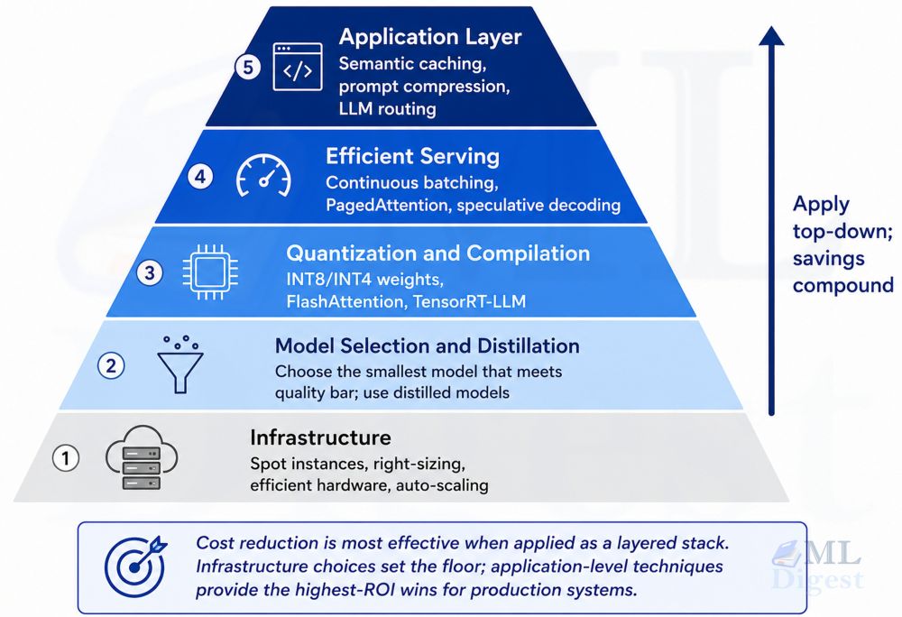
Here is a practical decision framework:
Start here (highest ROI, lowest effort):
- Switch to BF16 for training, INT8 or INT4 for inference
- Enable FlashAttention (it is one line of code in most frameworks)
- Use continuous batching (switch to vLLM)
- Add semantic caching for high-overlap query workloads
Next layer (medium effort, high savings):
- Apply LoRA or QLoRA instead of full fine-tuning
- Implement LLM routing between a cheap and expensive model
- Move training to spot/preemptible instances with checkpoint-based recovery
Advanced (high effort, significant savings at scale):
- Apply GPTQ or AWQ quantization for further inference compression
- Implement speculative decoding with a matched draft model
- Apply knowledge distillation to produce a task-specific smaller model
The right mix depends on your specific bottleneck. If your inference latency is the constraint, focus on speculative decoding and FlashAttention. If your monthly API bill is the constraint, start with routing and caching. If your fine-tuning runs are eating your GPU budget, go straight to QLoRA.
Summary
LLM costs are real, but they are not inevitable. Here is the one-paragraph version of this guide: train and fine-tune with mixed precision and PEFT (especially QLoRA); serve with quantized models using INT8/INT4, continuous batching via vLLM, and speculative decoding when latency matters; run on spot instances with frequent checkpointing; and at the application layer, add semantic caching and a routing layer to avoid calling expensive models when cheap ones will do.
The field is moving fast. Techniques like MoE (Mixture of Experts) routing at the model level, inference-time scaling through multi-token prediction, and hardware-aware model design are already reshaping the cost curve of the next generation of models. For a deeper look at the algorithmic side of this evolution, pushing the boundaries of LLM efficiency covers the latest research-driven advancements. But the fundamentals in this guide will remain useful: every layer of the stack is an opportunity to spend less and run more.

Happy is a seasoned ML professional with over 15 years of experience. His expertise spans various domains, including Computer Vision, Natural Language Processing (NLP), and Time Series analysis. He holds a PhD in Machine Learning from IIT Kharagpur and has furthered his research with postdoctoral experience at INRIA-Sophia Antipolis, France. Happy has a proven track record of delivering impactful ML solutions to clients. Check more about him here: https://sites.google.com/site/slhappyin/

Silpa brings 5 years of experience in working on diverse ML projects, specializing in designing end-to-end ML systems tailored for real-time applications. Her background in statistics (Bachelor of Technology) provides a strong foundation for her work in the field. Silpa is also the driving force behind the development of the content you find on this site.
Subscribe to our newsletter!