
Catastrophic forgetting occurs when sequential training on new data degrades a model’s performance on earlier tasks, domains, or capabilities. It is a core challenge in continual learning, where models must adapt without retraining from scratch.
The problem affects image classifiers, large language models (LLMs), diffusion models, forecasting systems, and personalized neural networks. This article explains why it happens, how to measure it, and how replay, regularization, distillation, and modular designs can reduce it.
1. The Problem in One Picture
A neural network stores many behaviors in the same parameters. When an optimizer improves the model on new data, it changes those shared parameters. Some changes are compatible with older behaviors, while others overwrite directions in parameter space that the old tasks relied on.
Consider two sequential image-classification tasks:
- Task $A$: distinguish cats from dogs.
- Task $B$: distinguish cars from trucks, using new data that arrives later.
After training on $A$, the model performs well on its validation set. If it is then trained only on $B$, it can improve on $B$ while its performance on $A$ falls sharply. The word catastrophic describes the size and speed of this regression, not a complete loss of every prior ability.
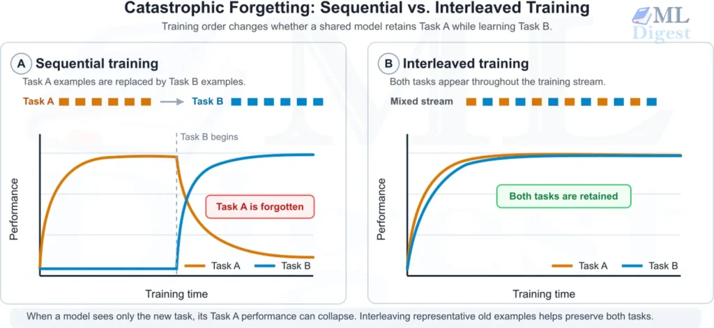
1.1 Forgetting is not every kind of performance drop
It is useful to separate catastrophic forgetting from nearby problems:
| Phenomenon | What changes? | Typical remedy |
|---|---|---|
| Catastrophic forgetting | Sequential training damages performance on earlier, still-relevant data | Replay, regularization, isolation, or distillation |
| Data drift | The input distribution changes | Monitoring, retraining, robust features |
| Concept drift | The relationship between inputs and targets changes | Time-aware evaluation, retraining, adaptation |
| Underfitting | The model cannot learn even the current task | More capacity, better optimization, better features |
| Negative transfer | Learning one task harms another during joint or transfer training | Task design, routing, balancing, isolation |
| Model degradation | Any sustained decline in deployed quality | Diagnose data, training, serving, and evaluation changes |
Drift often creates the business reason to update a model, while forgetting is the regression risk created by the update. Both may happen at once, especially in production time-series systems.
1.2 The learning setting changes what “retention” means
Continual-learning results are meaningful only when the evaluation setting is explicit. The commonly used task-, domain-, and class-incremental scenarios make different assumptions about what the model knows at inference time:
| Setting | What changes over time? | Is the task identity available at inference time? | Practical implication |
|---|---|---|---|
| Task-incremental learning | Tasks may have separate output heads or label spaces | Usually yes | Task-specific routing or heads can be valid |
| Domain-incremental learning | Inputs change, but the prediction task stays the same | No | The same predictor must work across domains |
| Class-incremental learning | New classes are added to one growing label space | No | Old and new classes must compete in one prediction head |
For a deployed system, define the unit of retention in product terms, such as language coverage, a safety behavior, a customer segment, a seasonal regime, or a class. A method that performs well with a known task identifier may not be suitable when production requests do not provide one.
1.3 A concrete example: cats, dogs, cars, and trucks
Suppose an image classifier first learns to distinguish cats from dogs. Its internal features learn to recognize fur texture, ears, snouts, and other useful signals. Next, it is trained extensively on cars versus trucks, with no animal images in the training batches. The network may repurpose some shared features to detect wheels, body shape, and windows. If those updates alter features that the animal classifier depended on, accuracy on cats versus dogs can fall even while accuracy on cars versus trucks rises.
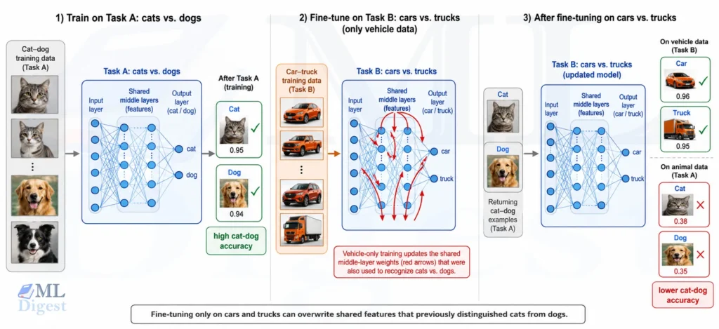
The three-panel visualization above represents this exact sequence: Task A is cats versus dogs, Task B is cars versus trucks, and the final red score is the lost animal-classification performance. The example is intentionally simple, but the same mechanism applies when a model moves from general text to a narrow professional corpus or from one seasonal demand regime to another.
The effect can be more obvious with a highly unrelated second task. If the same classifier is trained next to recognize handwritten digits instead of vehicles, its shared visual features and final decision layers receive gradients that are useful for strokes and digit shapes, not animal categories. Measure cat-versus-dog accuracy immediately before and after that digit-only training. A substantial drop, while digit accuracy rises, is direct evidence of catastrophic forgetting.
2. Why Neural Networks Forget
2.1 Gradient descent sees the present, not the past
Let $\phi$ be the model parameters and let $\mathcal{L}_B(\phi)$ be the loss on the current task. A standard gradient update is
$$
\phi_{t+1} = \phi_t – \eta \nabla_\phi \mathcal{L}_B(\phi_t),
$$
where $\eta$ is the learning rate. This update answers one narrow question: “Which small parameter change reduces the loss on the current batch?” It does not ask whether the same change raises the loss on task $A$.
At the point $\phi_A^*$ learned for task $A$, a small move $\Delta\phi$ changes the old loss approximately as
$$
\mathcal{L}_A(\phi_A^* + \Delta\phi)
\approx
\mathcal{L}_A(\phi_A^*) + \nabla \mathcal{L}_A(\phi_A^*)^\top\Delta\phi + \frac{1}{2}\Delta\phi^\top H_A\Delta\phi
$$
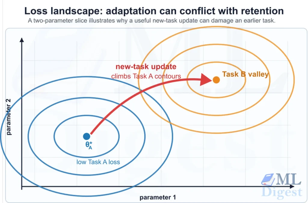
where $H_A$ is the curvature, or Hessian, of the old-task loss. Near a well-optimized solution, the first-order term is often small. The second-order term explains the danger: moving parameters along a high-curvature direction can rapidly increase the old loss. Yet task $B$ gradients can point exactly in such directions.
This is also why an apparently small fine-tuning run can cause a large regression. Parameter distance alone is not the whole story. A tiny change in an important direction can matter more than a much larger change in a flat direction.
Deep networks intentionally reuse features. Early layers may encode edges, word patterns, seasonal cycles, or denoising primitives that several tasks need. Sharing is data-efficient, but it couples tasks.
Interference is likely when:
- New training data is narrow, highly imbalanced, or very different from prior data.
- The model has limited spare capacity relative to the number of behaviors it must retain.
- Fine-tuning uses a large learning rate, many epochs, or updates all layers.
- Tasks use conflicting labels or objectives for similar inputs.
- The old data is unavailable, so training cannot measure the regression directly.
2.3 Distribution shift and missing historical data amplify the risk
When new data comes from a different distribution, the optimizer receives a stronger signal to change the model. A customer-support LLM updated only on a new product line, for example, may learn that new product’s terminology while losing coverage of older products. A time-series model trained only on a recent period can mistake a temporary regime for the whole world.
The problem becomes acute when earlier examples cannot be replayed. Without old inputs or another trustworthy retention signal, the update process has no direct way to observe that it is damaging a previously learned capability. Distribution shift is therefore not identical to catastrophic forgetting, but it frequently creates the conditions under which forgetting occurs.
3. How It Appears in Different Model Families
The mechanism is generic, but the visible failure depends on the model and objective.
3.1 LLMs and other autoregressive models
An LLM fine-tuned only on medical notes may gain domain vocabulary while losing instruction following, multilingual quality, safety behavior, or structured-output reliability. Fine-tuning can change reusable skills and response style as well as factual associations, so LLM performance degradation must be treated as an evaluation and release-management problem.
Keep representative prompts for capabilities that must remain stable, including safety-critical and tool-use cases, and evaluate them with task-specific checks rather than next-token loss alone. LoRA fine-tuning limits the updated weights but does not guarantee retention.
3.2 Do not confuse LLM forgetting with other failures
Several LLM failures can look similar in a product, but they have different causes and remedies:
| Failure | What it means | Why it is different from catastrophic forgetting |
|---|---|---|
| Catastrophic forgetting | A later update reduces a previously measured capability | It is caused by sequential adaptation and is demonstrated by before-and-after evaluation |
| Hallucination | The model generates unsupported or false content | It can occur in an unchanged model and does not require a prior capability to have regressed |
| Knowledge cutoff | The base model lacks information learned after its training data ended | The information was never reliably stored in that model, so it was not overwritten |
This distinction matters operationally. Retrieval can help with a knowledge cutoff, grounding and verification can reduce hallucinations, and retention tests plus continual-learning methods address catastrophic forgetting. A single failing prompt is not sufficient evidence that a model has forgotten.
3.3 Diffusion and other generative image models
Fine-tuning a diffusion model on a small set of product images or a new artistic style can improve concept fidelity while weakening diversity, prior concepts, or prompt alignment. For example, the model can begin to associate a common word with the newly learned subject too strongly. Methods such as DreamBooth use prior-preservation loss to reduce this type of language and image drift.
For a diffusion model, retain old prompts and judge outputs with both automated and human checks. Test style diversity, composition, and unwanted concept substitution, not only whether the new subject appears.
3.4 Time-series networks and streaming predictors
A forecasting network updated on the last few months of demand can adapt to a new promotion pattern and simultaneously forget seasonality from the previous year. An anomaly detector can adapt to a newly normal operating condition and lose sensitivity to an old, still-dangerous failure mode.
Time series makes replay design more subtle. Randomly mixing old windows can leak future information or break temporal relationships. Store time-consistent input-target windows, preserve rare events and seasonal regimes, and evaluate using rolling-origin splits. The principles in time-series forecasting remain essential while adding continual updates.
4. How to Measure Forgetting
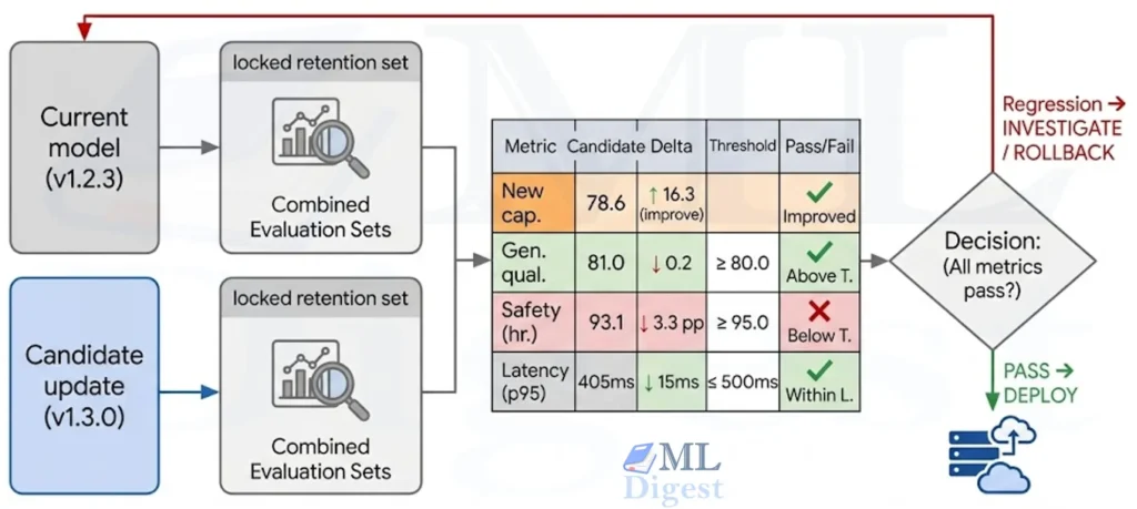
Measure forgetting by evaluating the same representative retention set before and after an update. Use a metric that fits the capability, such as accuracy for classification, forecast error for time series, or task-specific checks for an LLM. Record the score for each important capability, not only one overall average, because a useful average can hide a serious regression in a rare or safety-critical case.
For each release, report three things: whether the new capability improved, whether older capabilities stayed above their agreed thresholds, and whether serving costs such as latency or memory changed. Keep a locked test set separate from tuning data, compare the candidate with the current model, and investigate test-data, prompt, feature-pipeline, or label changes before concluding that training caused a regression.
5. Why Catastrophic Forgetting Matters
On a static benchmark, forgetting can look like a minor training artifact. In production, repeated updates for new data, users, markets, or policies can silently regress capabilities that users still depend on, making it a reliability risk.
- Continual learning: an always-improving system must absorb new information without resetting its useful history.
- Personalization: adapting a model to one user, language, or organization must not erase the general behavior that makes the model useful elsewhere.
- Robotics: a robot that learns a new floor plan or grasping routine must retain safe navigation and control skills from earlier environments.
- Autonomous systems: driving, warehouse, and industrial-control systems must adapt to new conditions without regressing on rare but safety-critical scenarios.
- Healthcare and other regulated settings: updates for new clinical data or instruments must not silently degrade performance for established patient groups and protocols.
- Fraud detection: a detector must learn new attack patterns without losing recall for known fraud strategies that appear only occasionally.
- Recommendation systems: models should incorporate new products and changing tastes while retaining useful preferences for long-tail users and items.
The risk is not that every old behavior must be preserved forever. Some knowledge becomes obsolete, incorrect, or inappropriate. The engineering goal is to distinguish intentional replacement from accidental loss, then make both choices observable and auditable.
6. Main Families of Defenses
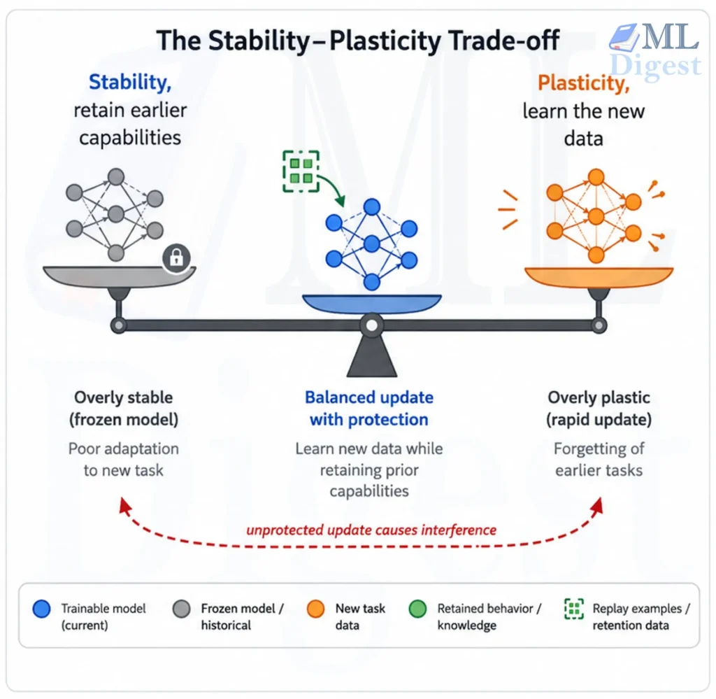
Continual learning is a balance between two desirable properties:
- Plasticity is the ability to absorb new information and improve on the current task.
- Stability is the ability to preserve useful behavior that earlier tasks established.
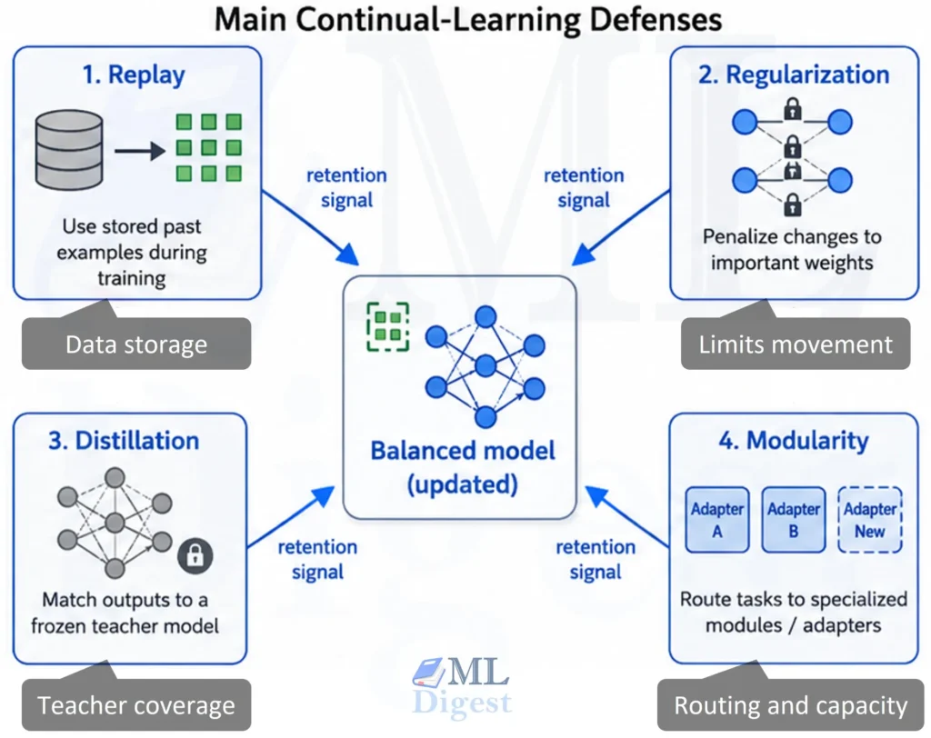
A model optimized only for plasticity can learn every new batch quickly and overwrite its past. A model optimized only for stability can preserve everything but fail to adapt when the world changes. Replay, EWC, distillation, and modularity are all different ways of finding a workable point on this trade-off. There is no universally correct balance, because the cost of an old-task regression and the value of rapid adaptation depend on the application.
In practice, robust systems often combine a small replay buffer with a lightweight retention penalty and careful evaluation.
6.1 Replay: practice old examples while learning new ones
Experience replay interleaves a small memory buffer $\mathcal{M}$ of earlier examples with current data. Its objective is simply joint training on a deliberately small approximation of history:
$$
\mathcal{L}(\theta) = \mathcal{L}_{\mathrm{new}}(\theta) + \lambda_{\mathrm{replay}}\mathcal{L}_{\mathcal{M}}(\theta).
$$
Replay is powerful because it gives the optimizer direct evidence of what must be retained. It works with classification, language modeling, diffusion denoising, regression, and forecasting, provided the stored examples reproduce the relevant old objective.
The limitations are equally concrete: raw examples can be costly, subject to privacy constraints, licensed for limited use, or unsuitable for long histories. Good buffers are diverse and balanced across tasks, classes, users, rare events, and temporal regimes. Random sampling is a useful baseline, but it can discard exactly the rare behavior you need to protect.
When raw data cannot be kept, consider approved embeddings, sufficient statistics, synthetic replay, or a frozen teacher that produces pseudo-targets. These alternatives reduce storage or privacy exposure, but can introduce their own bias and should be validated just as carefully.
6.2 Regularization: make important parameters expensive to change
Elastic Weight Consolidation (EWC) estimates how important each parameter was to an earlier task. After task $A$, it stores parameter values $\theta_A^*$ and importance weights $F_i$, commonly the diagonal of the Fisher information approximation. While learning task $B$, it uses
$$
\mathcal{L}_{\mathrm{EWC}}(\theta) = \mathcal{L}_B(\theta) + \frac{\lambda}{2}\sum_i F_i(\theta_i – \theta_{A,i}^*)^2.
$$
High-$F_i$ parameters are pulled toward their old values, while low-importance parameters remain relatively free to adapt. This turns the loss-landscape intuition into code.
EWC stores no raw examples, but its diagonal Fisher approximation can miss interactions between parameters and becomes harder to manage across many tasks. It is best treated as a useful baseline or a component of a broader solution, not a universal safeguard.
6.3 Knowledge distillation: preserve the old model’s behavior
With learning without forgetting, a frozen copy of the pre-update model acts as a teacher. On retained or unlabeled inputs $x$, minimize a discrepancy between its output distribution $p_{\mathrm{old}}(\cdot \mid x)$ and the new model distribution $p_\theta(\cdot \mid x)$:
$$
\mathcal{L}_{\mathrm{distill}} = \tau^2\operatorname{KL}\left( p_{\mathrm{old}}^{(\tau)}(\cdot \mid x)
\mathbin{|}
p_{\theta}^{(\tau)}(\cdot \mid x)
\right),
$$
where $\tau$ is a temperature that softens probabilities. Use this alongside the new task loss. For text and diffusion models, compare the outputs appropriate to the objective, such as token distributions, noise predictions, or intermediate representations.
Distillation can preserve useful dark knowledge in model outputs, but it cannot restore a capability if the teacher is already wrong or if the chosen inputs never exercise that capability. It also keeps the old model’s biases and failure modes.
6.4 Parameter isolation and modularity: allocate separate workspace
Isolation methods protect earlier behavior by reserving parameters or modules. Examples include task-specific heads, adapters, mixture-of-experts routing, learned masks, and progressively added modules. PackNet prunes and freezes weights for learned tasks, while parameter-efficient fine-tuning (PEFT) often keeps a base model frozen and trains a compact adapter.
Isolation is appealing when you need a stable base model, but it shifts the problem to routing, model-version management, and capacity growth. A separate adapter per customer or domain is only safe if inference reliably selects the right adapter and if shared components remain stable.
6.5 Adapter-based fine-tuning: change a small, explicit part of the model
Adapters, LoRA modules, and prompt-tuning components are practical forms of parameter isolation. They keep most of the base model frozen and train a small set of additional parameters. This can reduce update cost, simplify versioning, and make it easier to serve a stable base alongside several specialized variants.
However, an adapter does not automatically preserve behavior. It can alter outputs through the layers it modifies, an adapter may be applied to the wrong request, and merging it into the base weights removes the original separation. Treat an adapter as a controlled change surface, then evaluate the complete deployed model on its retention suite.
6.6 Architectural approaches: route work to compatible capacity
Architectures can reduce interference by assigning different inputs to different computation paths. A mixture-of-experts (MoE) model, for example, routes tokens or examples to a subset of expert modules. Modular networks, expandable networks, and dynamic architectures similarly add or select capacity for new tasks.
These approaches can protect specialized knowledge, but they introduce router errors, uneven expert use, extra memory, and harder deployment. They are most useful when tasks have a meaningful structure that a router can identify, rather than when every update is simply more data from the same distribution.
6.7 Comparing the major approaches
| Approach | Core idea | Main benefit | Main limitation |
|---|---|---|---|
| Replay | Revisit representative old data | Directly preserves old-task signals | Requires storage, governance, and careful sampling |
| Regularization | Penalize changes to important weights | Requires little or no raw old data | Can restrict useful adaptation and relies on approximate importance |
| Distillation | Match a frozen teacher’s outputs | Retains behavior on available inputs | Cannot preserve behavior that the teacher inputs do not cover |
| Parameter isolation | Reserve modules or weights by task | Reduces direct interference | Consumes capacity and needs reliable routing |
| Adapters | Train small modules around a stable base | Efficient customization and versioning | Does not eliminate output regressions |
| Dynamic architectures | Add or route to compatible capacity | Supports task specialization | Increases model and serving complexity |
6.8 Fine-tuning playbook: avoid forgetting before, during, and after an update
Fine-tuning is safest when it is treated as a constrained model update, not simply as additional training on the newest dataset. The following practices are complementary. A strong default is a curated replay set, a small parameter-efficient update, conservative optimization, and a release gate based on both the new and retained capabilities.
- Define what may change and what must remain stable. Write down the update’s target behavior, then select representative retention tests for the existing behaviors that matter. For an LLM, this may include instruction following, structured output, languages, safety cases, and tool use. For a diffusion model, use fixed prompt and seed grids. For a forecaster, preserve temporally valid windows from important seasonal and rare-event regimes.
- Mix new data with representative old data. Begin with a small, balanced replay buffer instead of fine-tuning on the new corpus alone. Include high-value edge cases, not only common examples. Tune the replay ratio on a development retention suite because too little old data does not protect the model, while too much can prevent the intended adaptation. If old data cannot be retained, use approved pseudo-labels or teacher outputs on a carefully chosen input set.
- Limit the update surface. Prefer adapters, LoRA, prompt tuning, or a selectively unfrozen subset of layers before updating every parameter. This limits the paths through which new gradients can alter established behavior and makes rollback and versioning simpler. It is a risk-reduction technique, not proof of retention, so test the final composed model rather than only the adapter in isolation.
- Use conservative optimization. Start from a lower learning rate and fewer epochs than a from-scratch training run, save frequent checkpoints, and stop when retention deteriorates even if the new-task loss continues to fall. Use a warmup and gradient clipping when appropriate to reduce destabilizing updates. Do not assume that more steps or a larger learning rate will make a narrow fine-tuning dataset more useful.
- Add an explicit preservation objective when the regression risk is high. Combine the new-task loss with replay loss, output distillation from the pre-update model, or an EWC-style penalty. The preservation term should be evaluated and tuned as a product constraint: a very strong penalty can block useful adaptation, while a weak one gives a false sense of security.
- Select and deploy with retention gates. Compare every candidate checkpoint with the pre-fine-tuning model on the locked retention suite and on the new task. Require per-capability thresholds, not only a better aggregate score. Keep the previous model, the data snapshot, the evaluation report, and a rollback path until post-deployment monitoring confirms that the update behaves as expected.
This playbook does not guarantee zero regression. It makes the trade-off visible early, enables a controlled rollback, and reduces the chance that a narrow adaptation silently overwrites an important general capability.
7. A Practical PyTorch Baseline: Replay Plus EWC-Style Regularization
The following PyTorch example is deliberately model-agnostic. It works for any model whose training objective returns a differentiable scalar loss. The old_batch can contain classification samples, token sequences, diffusion training tuples, or time-series windows. The key idea is always the same: optimize new data while explicitly retaining an old-data signal and discouraging harmful parameter drift.
import torch
from torch import nn


class RetentionTrainer:
    """Add replay and an EWC-style penalty to an ordinary PyTorch model."""

    def __init__(self, model: nn.Module, loss_fn, optimizer, ewc_weight: float = 10.0):
        self.model = model
        self.loss_fn = loss_fn
        self.optimizer = optimizer
        self.ewc_weight = ewc_weight
        self.reference_params = {}
        self.importance = {}

    def snapshot_parameters(self) -> None:
        """Save the model state at the end of a task or approved model version."""
        self.reference_params = {
            name: parameter.detach().clone()
            for name, parameter in self.model.named_parameters()
            if parameter.requires_grad
        }

    def estimate_importance(self, calibration_batches) -> None:
        """Estimate diagonal Fisher importance from representative old-data batches.

        Each batch is a (features, targets) tuple. For generative models, adapt
        `loss_fn` so targets contain the model-specific training target.
        """
        self.importance = {
            name: torch.zeros_like(parameter)
            for name, parameter in self.model.named_parameters()
            if parameter.requires_grad
        }

        batch_count = 0
        self.model.eval()
        for features, targets in calibration_batches:
            self.optimizer.zero_grad(set_to_none=True)
            loss = self.loss_fn(self.model(features), targets)
            loss.backward()

            for name, parameter in self.model.named_parameters():
                if parameter.grad is not None and name in self.importance:
                    self.importance[name] += parameter.grad.detach().square()
            batch_count += 1

        for name in self.importance:
            self.importance[name] /= max(batch_count, 1)

        self.model.train()

    def retention_penalty(self) -> torch.Tensor:
        """Penalize changes to parameters important to the previous task."""
        if not self.reference_params or not self.importance:
            return torch.zeros((), device=next(self.model.parameters()).device)

        penalty = torch.zeros((), device=next(self.model.parameters()).device)
        for name, parameter in self.model.named_parameters():
            if name in self.importance:
                delta = parameter - self.reference_params[name]
                penalty = penalty + (self.importance[name] * delta.square()).sum()
        return 0.5 * self.ewc_weight * penalty

    def train_step(self, new_batch, old_batch=None, replay_weight: float = 1.0):
        """Train once on current data and, when available, a replay batch."""
        self.model.train()
        self.optimizer.zero_grad(set_to_none=True)

        new_features, new_targets = new_batch
        loss = self.loss_fn(self.model(new_features), new_targets)

        if old_batch is not None:
            old_features, old_targets = old_batch
            replay_loss = self.loss_fn(self.model(old_features), old_targets)
            loss = loss + replay_weight * replay_loss

        loss = loss + self.retention_penalty()
        loss.backward()
        self.optimizer.step()
        return loss.detach()


def make_task(sign: float, sample_count: int = 256):
    """Create two related binary tasks with conflicting decision boundaries."""
    features = torch.randn(sample_count, 2)
    targets = (features[:, 0] + sign * features[:, 1] > 0).long()
    return features, targets


@torch.no_grad()
def accuracy(model: nn.Module, batch) -> float:
    features, targets = batch
    return (model(features).argmax(dim=1) == targets).float().mean().item()


torch.manual_seed(42)
task_a = make_task(sign=1.0)
task_b = make_task(sign=-1.0)

model = nn.Sequential(nn.Linear(2, 16), nn.ReLU(), nn.Linear(16, 2))
trainer = RetentionTrainer(
    model=model,
    loss_fn=nn.CrossEntropyLoss(),
    optimizer=torch.optim.Adam(model.parameters(), lr=0.01),
    ewc_weight=20.0,
)

# Learn Task A, then save the parameter values and their estimated importance.
for _ in range(100):
    trainer.train_step(task_a)
trainer.snapshot_parameters()
trainer.estimate_importance([task_a])
print(f"After Task A: A={accuracy(model, task_a):.3f}, B={accuracy(model, task_b):.3f}")

# Learn Task B while replaying a randomly chosen old-data minibatch from Task A.
for _ in range(100):
    indices = torch.randint(len(task_a[0]), size=(64,))
    replay_batch = (task_a[0][indices], task_a[1][indices])
    trainer.train_step(task_b, old_batch=replay_batch, replay_weight=1.0)
print(f"After Task B: A={accuracy(model, task_a):.3f}, B={accuracy(model, task_b):.3f}")

# Expected output:
#     After Task A: A=0.992, B=0.445
# After Task B: A=0.719, B=0.746The two synthetic tasks deliberately compete, so the exact scores will vary, but Task A should remain substantially stronger after learning Task B than it would with Task B-only training. To measure the benefit, run the same experiment with old_batch=None and ewc_weight=0.0. This is a teaching baseline, not a production framework. In a real system, preserve device placement in the data pipeline, choose a model-appropriate loss function, and estimate importance on a held-out sample that represents the capabilities you must retain. For many prior tasks, you may accumulate, decay, or compress importance estimates instead of retaining a snapshot for every task.
8. A Safe Update Workflow
- Define protected capabilities. Before training, turn “do not forget” into a testable contract. Define the representative inputs, metrics, acceptable regression, owner, and escalation path. Avoid unbounded requirements such as “retain all pretraining knowledge.”
- Construct the retention set. Build a compact evaluation suite and, where permitted, a separate replay set that cover normal traffic, high-cost edge cases, and relevant historical regimes. Use deterministic and adversarial checks for LLMs, fixed prompt-and-seed grids for diffusion models, and temporally valid windows for time series. Tune on a development set, then make the release decision on a separate locked test set.
- Train conservatively and compare checkpoints. Start with a low learning rate, short updates, and frequent checkpoints. Tune replay and regularization on the development suite, compare every candidate with the production model on new and retained capabilities, and keep the previous model ready for rollback.
- Monitor after deployment. Offline tests are necessary but not sufficient. Monitor slice-level quality, distribution change, calibration, latency, and user feedback. Use MLflow to link model versions, data, evaluations, and releases, and OpenTelemetry for serving traces and metrics. Pause updates or roll back when a regression crosses its threshold.
9. Common Mistakes
- “More epochs will make the new skill stick.” More epochs on narrow new data can intensify forgetting. Improvement on the update dataset is not proof that the update is safe. Use early stopping based on both adaptation and retention metrics.
- “Freezing layers eliminates forgetting.” Freezing can protect some representations, but trainable layers can still alter outputs enough to harm behavior. It can also prevent necessary adaptation. Measure retained capabilities instead of assuming a particular freeze pattern is protective.
- “A small replay buffer is automatically representative.” A buffer built from the most recent or most common examples will often forget rare classes, languages, seasonal peaks, and safety cases. Define sampling strata explicitly and inspect the buffer as a dataset.
- “One aggregate score is enough.” An average can improve while an essential slice fails. Report per-task, per-domain, and worst-case results. If a metric is noisy, include confidence intervals or repeated evaluation rather than treating small differences as meaningful.
- “Parameter-efficient fine-tuning means risk-free fine-tuning.” Adapters reduce the number of trainable parameters and simplify versioning, but an adapter can still change output behavior substantially. Test the deployed composition, including adapter selection, merge behavior, quantization, prompts, and inference settings.
10. Current Challenges and Open Questions
The main techniques work, but difficult questions remain:
- How much history is enough? A replay buffer must balance retention, storage cost, privacy, and the rarity of critical cases.
- What should a model intentionally forget? Removing stale or incorrect information is different from accidental forgetting. Machine unlearning studies how to remove the influence of selected training data, but reliable verification remains challenging, particularly under privacy and data-governance constraints.
- Which behavior is important? Parameter importance, teacher outputs, and benchmark examples are only proxies for the capabilities a system should retain.
- Can continual learning scale? Foundation models make replay, importance estimation, multi-model distillation, and extensive evaluation expensive.
- How can memory be made efficient? Practical lifelong-learning systems need compact buffers, summaries, or learned retrieval mechanisms that preserve critical coverage without storing every historical example.
- Which benchmarks reflect real use? Many task-sequence benchmarks are useful but simplified. Better evaluations should include long streams, changing distributions, realistic privacy constraints, and both adaptation and retention costs.
- How should conflicting goals be resolved? When a new policy should replace an old behavior, no algorithm can infer the correct product decision. Teams need explicit requirements, versioned evaluations, and a safe rollout process.
These questions move catastrophic forgetting beyond an optimization problem. It is also a data-governance, evaluation, and deployment problem.
11. The Future of Continual Learning
The long-term goal is lifelong learning: systems that acquire useful skills over extended periods, selectively revise obsolete knowledge, and remain dependable on retained capabilities. Progress will likely come from combinations rather than a single universal technique. For example, a system may use compact, privacy-aware replay for representative history, distillation to preserve broad behavior, adapters or experts for specialization, and regularization for particularly sensitive parameters.
More modular architectures can give new knowledge a controlled place to live, while efficient memory and retrieval mechanisms can make retention feasible on edge devices and at foundation-model scale. Equally important, better benchmarks and release evaluations must measure stability, plasticity, compute, privacy, and safety together. The most useful continual-learning method is not simply the one with the lowest average forgetting, but the one that satisfies the relevant retention contract within operational constraints.
Summary
Catastrophic forgetting happens because sequential gradient updates optimize the present task through parameters that also encode past behavior. It affects classifiers, LLMs, diffusion models, and time-series networks alike. The practical response is to make retention explicit: preserve representative tests, measure score changes after every update, and give training an old-task signal through replay, regularization, distillation, modularity, or a combination of them.
Start with one upcoming model update. Define three to ten capabilities that must remain stable, create a small temporally and semantically representative retention set, run the current model and the fine-tuned candidate side by side, and record the trade-off. That modest discipline turns catastrophic forgetting from a late-stage surprise into an engineering decision you can measure and control.

Happy is a seasoned ML professional with over 15 years of experience. His expertise spans various domains, including Computer Vision, Natural Language Processing (NLP), and Time Series analysis. He holds a PhD in Machine Learning from IIT Kharagpur and has furthered his research with postdoctoral experience at INRIA-Sophia Antipolis, France. Happy has a proven track record of delivering impactful ML solutions to clients. Check more about him here: https://sites.google.com/site/slhappyin/

Silpa brings 5 years of experience in working on diverse ML projects, specializing in designing end-to-end ML systems tailored for real-time applications. Her background in statistics (Bachelor of Technology) provides a strong foundation for her work in the field. Silpa is also the driving force behind the development of the content you find on this site.
Subscribe to our newsletter!