Retrieval-Augmented Generation (RAG): A Practical Guide

Retrieval-Augmented Generation (RAG) is a technique that acts as an open-book exam for Large Language Models (LLMs). It allows a model to browse external data references at query time, rather than relying solely on its static training memory.

The Intuition: The Open-Book Exam

Imagine you are a student sitting for a final exam in Advanced Quantum Physics.

• Scenario A (Pure LLM): You are taking a closed-book exam. You must rely entirely on what you memorized during your studies months ago. If you forgot a specific constant or a recent formula, you might hallucinate a plausible-sounding but incorrect answer to fill the gap.
• Scenario B (RAG): You are taking an open-book exam. You are allowed to carry a textbook and a notebook into the hall. When a question asks about a specific experiment, you do not just guess; you look up the exact page, read the relevant paragraph, and then synthesize the answer.

RAG transforms the LLM from Scenario A to Scenario B. It gives the model access to a dynamic library of information that it can search, read, and use to generate accurate responses.

In this guide, we will explore the architecture of RAG, the mathematics behind the retrieval mechanism, and the code required to build it.

1. Why RAG?

1.1 The Limitations of Fixed Weights

Large Language Models are powerful reasoning engines, but when used in isolation, they suffer from significant memory limitations:

• Fixed Knowledge Cutoff: A model only knows what it saw during its training. It is unaware of events or documents created after that date.
• Hallucinations: When a model is unsure, it often prioritizes fluency over factuality, generating confident but wrong assertions.
• High Update Costs: Updating a model’s internal knowledge requires retraining or extensive fine-tuning, which is computationally expensive and slow.
• Opacity: It can be difficult to trace why a model produced a specific answer, or to provide auditable sources.

These limitations become acute in real systems where:

• Content changes frequently (documentation, policies, product catalogs).
• Compliance and traceability matter (finance, healthcare, legal).
• You must reduce hallucinations and provide citations.

1.2 The Strategic Value of RAG

RAG is not merely “adding a vector database.” It is a separation of concerns:

• Knowledge storage lives in your corpus and index.
• Reasoning and writing live in the LLM.

This separation is operationally important: you update the corpus without retraining the model.

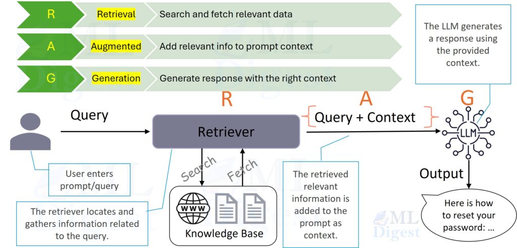
1.3 The Core Idea of RAG

RAG addresses these problems by decoupling knowledge storage from reasoning:

• The Retriever acts as the librarian. It finds the relevant pages from a knowledge base (like a vector database).
• The Generator acts as the writer. It takes the user’s question and the retrieved pages, then synthesizes an answer.

High-level data flow:

1. Query: The user asks a question $q$.
2. Search: The system searches a large corpus $\mathcal{C}$ for the top-$k$ most relevant chunks.
3. Augment: The system feeds both the question $q$ and the retrieved chunks into the LLM.
4. Generate: The LLM generates a response grounded in the retrieved text.

This architecture makes systems maintainable. If your company updates its vacation policy, you simply update the document in the database. You do not need to retrain the neural network.

2. High-Level RAG Architecture

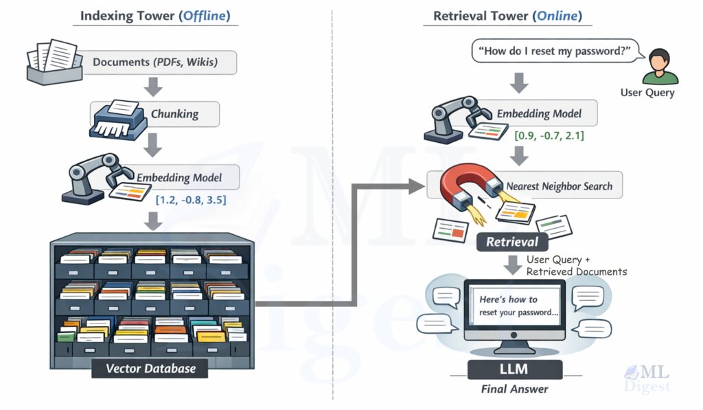
It is useful to separate RAG into two pipelines: an offline indexing pipeline (prepare the corpus) and an online retrieval + generation pipeline (answer user queries).

2.1 RAG Flow

In the above figure, the two vertical “towers” are connected by a shared embedding space.

• The indexing tower turns documents into vectors and stores them.
• The retrieval tower turns the user query into a vector, finds nearby vectors, and hands the matching text to the LLM.

The Indexing Tower (Offline)

1. Documents: You start with your knowledge base (PDFs, Wikis, HTML pages).
2. Chunking: You slice these documents into small, digestible semantic units—like paragraphs in a textbook.
3. Embedding: You pass these chunks through an Embedding Model, which converts text into a vector (a list of numbers).
4. Index: You store these vectors in a Vector Database, creating a geometric map of your knowledge.

The Retrieval Tower (Online)

1. User Query: A user asks, “How do I reset my password?”
2. Query Embedding: The same Embedding Model converts this question into a vector.
3. Nearest Neighbor Search: The database calculates the distance between the question-vector and all document-vectors, finding the closest matches.
4. Generation: The LLM receives the prompt: “Context: [Retrieved Chunks]. User Question: [Query]. Answer:”

2.2 Key Components

• Orchestrator: Application code (framework or custom) that manages ingestion, retrieval, prompt construction, and citations.
• Retriever: The search component, typically:
  • Embedding model: Converts text to vectors (for example, modern bge / E5 / GTE families).
  • Vector store: Performs nearest-neighbor search (FAISS, Qdrant, Pinecone, pgvector).
• Generator: The LLM that synthesizes the final answer.

2.3 A Minimal “Prompt Contract” (Grounding Rule)

In practice, much of RAG quality comes from a simple contract you enforce in the prompt:

• Use the retrieved context as the primary evidence.
• If the answer is not supported by the retrieved context, say that the evidence is insufficient.
• When possible, cite or quote the specific passages used.

This contract turns retrieval into a measurable bottleneck: if the retriever fails to surface the relevant passage, the generator should not guess.

3. Mathematical View

Let us formalize the retrieval and generation steps.

3.1 Offline Pipeline: Indexing

RAG is easiest to reason about when you separate what happens before any user question (offline) from what happens at question time (online).

The offline pipeline builds a search structure over your corpus.

1. Documents: Let $\mathcal{D} = \{d_1, \ldots, d_M\}$ be the raw documents.
2. Chunking: A chunker splits each document into smaller, atomic units (passages) so we can retrieve precise information later:

$$
g(d_i) = (z_{i,1}, \ldots, z_{i,n_i}).
$$

Let the full chunk set be $\mathcal{C} = \bigcup_{i=1}^{M} \{z_{i,1}, \ldots, z_{i,n_i}\}$.

3. Embedding: An embedding model $f_\phi$ maps each chunk to a vector:

$$
e(z) = f_\phi(z) \in \mathbb{R}^d.
$$

4. Indexing: An index $\mathcal{I}$ stores all chunk embeddings (plus metadata) to support fast nearest-neighbor search:

$$
\mathcal{I} \leftarrow \operatorname{BuildIndex}(\{(e(z), z) : z \in \mathcal{C}\}).
$$

3.2 Online Pipeline: Retrieval + Generation

Given a user query $q$, the system:

1. Embeds the query: $e(q) = f_\phi(q)$.
2. Retrieves evidence: query the index for top-$k$ chunks.
3. Generates an answer: condition the language model on the query plus the retrieved chunks.

The rest of this section makes steps (2) and (3) more explicit.

3.2.1 The Retrieval Space

The relevance score $s(q, z)$ is commonly defined by the dot product or cosine similarity between vectors:

$$
s(q, z) = \frac{f_\phi(q)^\top f_\phi(z)}{|f_\phi(q)| |f_\phi(z)|}
$$

The retriever selects the Top-$k$ chunks ($\mathcal{Z}_k$) that maximize this score:

$$
\mathcal{Z}_k = \operatorname*{Top-k}_{z \in \mathcal{C}} s(q, z)
$$

You can also express retrieval as an (approximate) distribution over chunks, for example by normalizing scores with a softmax:

$$
P(z \mid q) = \frac{\exp(\beta\, s(q, z))}{\sum_{z’ \in \mathcal{C}} \exp(\beta\, s(q, z’))}
$$

where $\beta$ is a temperature parameter. In practice, this distribution is approximated by restricting the denominator to the retrieved set $\mathcal{Z}_k$.

3.2.2 Probabilistic Generation

Standard language modeling estimates the probability of a sequence $y$ given an input $q$:

$$
P(y \mid q)
$$

In RAG, we treat the retrieved document $z$ as a latent variable. In our student analogy, this corresponds to the probability of selecting a specific book $z$ from the shelf to answer the question. The generation probability marginalizes over all possible documents. Ideally, we would sum over all passages in the corpus:

$$
P(y \mid q) = \sum_{z \in \mathcal{C}} P(y \mid q, z) P(z \mid q)
$$

However, summing over the entire corpus $\mathcal{C}$ is computationally intractable. In practice, we approximate this sum using the top-$k$ retrieved documents $\mathcal{Z}_k$:

$$
P(y \mid q) \approx \sum_{z \in \mathcal{Z}_k} P(y \mid q, z) P(z \mid q)
$$

• $P(z \mid q)$ represents retrieval confidence (often a normalized score).
• $P(y \mid q, z)$ represents the generator probability given the query and a specific passage.

In many implementations, the system concatenates the top-$k$ passages into a single context block $c = [z_1; \dots; z_k]$ and conditions generation on that block:

$$
y \sim P(y \mid q, c)
$$

This mathematical view highlights the core improvement RAG offers: we represent the probability of an answer not just as a function of the model’s weights $\theta$, but as a function of the explicitly retrieved context $c$.

4. Building Blocks in Practice

In this section, we connect the concepts to concrete implementation steps.

The components are: Ingest Documents → Clean → Chunk → Annotate → Embed → Index → Retrieve → Prompt Construction → Generate Output.

System:
You are a helpful assistant. Follow the rules strictly.

Rules:
1) Use only the Sources for factual claims.
2) If the Sources do not contain enough evidence, say: "The evidence is insufficient."
3) Cite sources using brackets like [docA#chunk12].
4) Do not invent citations.

Sources:
1. [docA#chunk12] (Title: ..., Section: ...)
    ...chunk text...
2. [docB#chunk03] (Title: ..., Section: ...)
    ...chunk text...

User Question:
...user question...

Answer:

Answer format:
- Short answer (1-2 sentences)
- Evidence bullets (each bullet must include a citation)

When you cite a source, include a short quote (one sentence) from that source.
Format: Claim ... [docA#chunk12: "quoted sentence"]

from __future__ import annotations

from dataclasses import dataclass
from typing import List, Optional

!pip install faiss-cpu
import faiss
import numpy as np
from sentence_transformers import SentenceTransformer


@dataclass(frozen=True)
class Chunk:
    chunk_id: str
    doc_id: str
    heading: str
    text: str


class SimpleRAG:
    """A minimal, runnable RAG skeleton: chunk -> embed -> search -> prompt."""

    def __init__(self, model_name: str = "sentence-transformers/all-MiniLM-L6-v2"):
        self.encoder = SentenceTransformer(model_name)
        self.chunks: List[Chunk] = []
        self.index: Optional[faiss.Index] = None

    def build_index(self, documents: List[tuple[str, str]], chunk_size: int = 120, overlap: int = 20) -> None:
        """Build an in-memory FAISS index over (doc_id, text) documents."""
        self.chunks = self._chunk_documents(documents, chunk_size=chunk_size, overlap=overlap)

        texts = [c.text for c in self.chunks]
        embeddings = self.encoder.encode(texts, convert_to_numpy=True, show_progress_bar=True)

        # Normalize for cosine similarity via inner product.
        faiss.normalize_L2(embeddings)

        d = embeddings.shape[1]
        self.index = faiss.IndexFlatIP(d)
        self.index.add(embeddings)

    def retrieve(self, query: str, top_k: int = 5) -> List[tuple[Chunk, float]]:
        if self.index is None:
            raise ValueError("Index is not built. Call build_index first.")

        q_emb = self.encoder.encode([query], convert_to_numpy=True)
        faiss.normalize_L2(q_emb)

        scores, indices = self.index.search(q_emb, top_k)

        results: List[tuple[Chunk, float]] = []
        for score, idx in zip(scores[0], indices[0]):
            if idx == -1:
                continue
            results.append((self.chunks[int(idx)], float(score)))
        return results

    def generate_prompt(self, query: str, retrieved: List[tuple[Chunk, float]]) -> str:
        sources = []
        for chunk, _score in retrieved:
            sources.append(
                f"[{chunk.chunk_id}] ({chunk.doc_id} · {chunk.heading})\n{chunk.text}"
            )

        sources_block = "\n\n".join(sources)
        return (
            "You are a helpful assistant. Answer the question using only the sources below.\n"
            "If the sources do not contain enough evidence, state that the evidence is insufficient.\n\n"
            "Sources:\n"
            f"{sources_block}\n\n"
            f"Question: {query}\n"
            "Answer with citations like [chunk_id]."
        )

    def _chunk_documents(
        self, documents: List[tuple[str, str]], chunk_size: int, overlap: int
    ) -> List[Chunk]:
        """Simple word-window chunker with stable chunk ids and lightweight metadata."""
        if chunk_size <= overlap:
            raise ValueError("chunk_size must be larger than overlap")

        chunks: List[Chunk] = []
        step = chunk_size - overlap
        for doc_id, heading, text in documents:
            words = text.split()
            for start in range(0, len(words), step):
                window = words[start : start + chunk_size]
                if not window:
                    continue
                chunk_index = len(chunks)
                chunk_id = f"{doc_id}#chunk{chunk_index:04d}"
                chunks.append(
                    Chunk(
                        chunk_id=chunk_id,
                        doc_id=doc_id,
                        heading=heading,
                        text=" ".join(window),
                    )
                )
        return chunks


if __name__ == "__main__":
    # Each document is (doc_id, text). In production, doc_id would map to a URL or file.
    docs = [
        (
            "docA", "titleA",
            "RAG helps LLM applications by retrieving external text at query time and grounding answers on that text.",
        ),
        (
            "docB", "titleB",
            "Fine-tuning updates a model weights using additional training data; it is useful for behavior and style but is costly to keep current.",
        ),
    ]

    rag = SimpleRAG()
    rag.build_index(docs)

    query = "How does RAG help LLM applications?"
    retrieved = rag.retrieve(query, top_k=2)
    prompt = rag.generate_prompt(query, retrieved)

    print(prompt)

from __future__ import annotations

from dataclasses import dataclass
from typing import List, Optional

!pip install faiss-cpu
import faiss
import numpy as np
from sentence_transformers import SentenceTransformer


@dataclass(frozen=True)
class Chunk:
    chunk_id: str
    doc_id: str
    heading: str
    text: str


class SimpleRAG:
    """A minimal, runnable RAG skeleton: chunk -> embed -> search -> prompt."""

    def __init__(self, model_name: str = "sentence-transformers/all-MiniLM-L6-v2"):
        self.encoder = SentenceTransformer(model_name)
        self.chunks: List[Chunk] = []
        self.index: Optional[faiss.Index] = None

    def build_index(self, documents: List[tuple[str, str]], chunk_size: int = 120, overlap: int = 20) -> None:
        """Build an in-memory FAISS index over (doc_id, text) documents."""
        self.chunks = self._chunk_documents(documents, chunk_size=chunk_size, overlap=overlap)

        texts = [c.text for c in self.chunks]
        embeddings = self.encoder.encode(texts, convert_to_numpy=True, show_progress_bar=True)

        # Normalize for cosine similarity via inner product.
        faiss.normalize_L2(embeddings)

        d = embeddings.shape[1]
        self.index = faiss.IndexFlatIP(d)
        self.index.add(embeddings)

    def retrieve(self, query: str, top_k: int = 5) -> List[tuple[Chunk, float]]:
        if self.index is None:
            raise ValueError("Index is not built. Call build_index first.")

        q_emb = self.encoder.encode([query], convert_to_numpy=True)
        faiss.normalize_L2(q_emb)

        scores, indices = self.index.search(q_emb, top_k)

        results: List[tuple[Chunk, float]] = []
        for score, idx in zip(scores[0], indices[0]):
            if idx == -1:
                continue
            results.append((self.chunks[int(idx)], float(score)))
        return results

    def generate_prompt(self, query: str, retrieved: List[tuple[Chunk, float]]) -> str:
        sources = []
        for chunk, _score in retrieved:
            sources.append(
                f"[{chunk.chunk_id}] ({chunk.doc_id} · {chunk.heading})\n{chunk.text}"
            )

        sources_block = "\n\n".join(sources)
        return (
            "You are a helpful assistant. Answer the question using only the sources below.\n"
            "If the sources do not contain enough evidence, state that the evidence is insufficient.\n\n"
            "Sources:\n"
            f"{sources_block}\n\n"
            f"Question: {query}\n"
            "Answer with citations like [chunk_id]."
        )

    def _chunk_documents(
        self, documents: List[tuple[str, str]], chunk_size: int, overlap: int
    ) -> List[Chunk]:
        """Simple word-window chunker with stable chunk ids and lightweight metadata."""
        if chunk_size <= overlap:
            raise ValueError("chunk_size must be larger than overlap")

        chunks: List[Chunk] = []
        step = chunk_size - overlap
        for doc_id, heading, text in documents:
            words = text.split()
            for start in range(0, len(words), step):
                window = words[start : start + chunk_size]
                if not window:
                    continue
                chunk_index = len(chunks)
                chunk_id = f"{doc_id}#chunk{chunk_index:04d}"
                chunks.append(
                    Chunk(
                        chunk_id=chunk_id,
                        doc_id=doc_id,
                        heading=heading,
                        text=" ".join(window),
                    )
                )
        return chunks


if __name__ == "__main__":
    # Each document is (doc_id, text). In production, doc_id would map to a URL or file.
    docs = [
        (
            "docA", "titleA",
            "RAG helps LLM applications by retrieving external text at query time and grounding answers on that text.",
        ),
        (
            "docB", "titleB",
            "Fine-tuning updates a model weights using additional training data; it is useful for behavior and style but is costly to keep current.",
        ),
    ]

    rag = SimpleRAG()
    rag.build_index(docs)

    query = "How does RAG help LLM applications?"
    retrieved = rag.retrieve(query, top_k=2)
    prompt = rag.generate_prompt(query, retrieved)

    print(prompt)

You are a helpful assistant. Answer the question using only the sources below.
If the sources do not contain enough evidence, state that the evidence is insufficient.

Sources:
[docA#chunk0000] (docA · titleA)
RAG helps LLM applications by retrieving external text at query time and grounding answers on that text.

[docB#chunk0001] (docB · titleB)
Fine-tuning updates a model weights using additional training data; it is useful for behavior and style but is costly to keep current.

Question: How does RAG help LLM applications?
Answer with citations like [chunk_id].

5. Variants and Extensions of RAG

The basic RAG pattern (single-step retrieve-then-generate) is powerful, but many real systems use more sophisticated variants.

5.1 Multi-Stage and Hybrid Retrieval

To improve recall and precision, you can:

• Hybrid retrieval
  • Combine dense retrieval (embeddings) with sparse retrieval (BM25, keyword search).
  • Example: score = alpha * dense_score + (1 - alpha) * sparse_score.
• Reranking
  • First retrieve a larger set (e.g., top-100) with a fast method.
  • Then use a cross-encoder or reranker model to rescore the candidates and choose the top-k to feed into the LLM.
• Metadata-aware retrieval
  • Filter by structured metadata (date, language, customer id).

Why Reranking Helps (Intuition)

Dense retrieval is fast and good at semantic recall, but it can mis-rank passages that share “topic words” without containing the precise answer. A reranker (often a cross-encoder) reads the query and a candidate passage together and produces a more faithful relevance score.

In practice, a strong baseline is:

1. Retrieve top-50 to top-200 candidates with a fast retriever.
2. Rerank with a cross-encoder.
3. Send top-3 to top-10 to the generator.

5.2 Iterative / Conversational RAG

In conversational settings, you often want to:

• Incorporate chat history alongside retrieved documents.
• Perform follow-up retrieval based on intermediate results.

Example flow:

1. Use the latest user message and some history as the query.
2. Retrieve context and answer.
3. If the model detects that information is missing, it may issue another retrieval (sometimes guided by tool calls or special prompts).

5.3 Agentic RAG and Tools

In more advanced systems, the LLM acts as an agent that can:

• Decide when to call a retriever tool.
• Decide which collection or index to query.
• Possibly call other domain-specific tools (search APIs, databases, calculators) and combine the results.

The core idea remains the same: ground the model’s reasoning in external, query-time information.

5.4 Structured Outputs and RAG

RAG is not limited to free-form text answers. You can combine retrieval with:

• JSON schemas or function-calling to get structured output.
• SQL generation where the model consults retrieved table schemas or documentation.
• Code generation where retrieval provides relevant code snippets or API docs.

6. Design Choices and Trade-Offs

Designing a good RAG system involves many practical decisions. Here are key axes to consider.

6.1 Chunk Size and Overlap

• Small chunks (e.g., 100–300 tokens):
  • Pros: fine-grained retrieval; less irrelevant text.
  • Cons: loss of semantic context; may miss context that spans multiple chunks.
• Large chunks (e.g., 800–2000 tokens):
  • Pros: more context per retrieval; preserves narrative flow and context; fewer queries to index.
  • Cons: higher cost per query (more tokens to LLM); risk of noise; “Lost-in-the-middle” phenomenon (LLMs struggle to find facts in the middle of long contexts).

Common practice: start with 300–800 tokens with 10–20% overlap and tune empirically.

6.2 Number of Retrieved Chunks (k)

• Low k (e.g., 3–5):
  • Pros: smaller prompts; cleaner context for the LLM; faster and cheaper.
  • Cons: lower recall; may miss some relevant content.
• High k (e.g., 10–40):
  • Pros: higher recall; better coverage.
  • Cons: more noise; longer prompts; possible confusion/hallucination for the LLM; higher cost.

The optimal k depends on:

• Query complexity
• Domain size and redundancy
• Model context window and cost constraints

6.3 Embedding Model Choice

• Smaller, faster embeddings (e.g., 384–768 dimensions):
  • Cheaper to compute, smaller index, faster search.
  • Adequate for many enterprise QA use cases.
• Larger, more expressive embeddings (e.g., 1,024–4,096 dimensions):
  • Better semantic fidelity and cross-lingual performance.
  • More expensive compute and storage.

It is common to start with a good open model (e.g., a modern bge / GTE / E5 model) and only move to heavier models if quality is insufficient.

6.4 Vector Store and Indexing Strategy

Consider:

• Scale: How many chunks (10k vs 10M+) do you need to store?
• Latency: Do you need sub-100ms retrieval?
• Filtering: Do you need complex metadata filters or hybrid search?
• Operational complexity: Self-hosted vs fully managed.

Do not over-engineer the database on Day 1.

• For < 100k chunks: An in-memory index (like FAISS or even a local array) is faster and simpler than managing a dedicated server.
• For > 1M chunks: You need a managed Vector Database (Pinecone, Qdrant, Weaviate, pgvector) to handle persistence, replication, and filtering at scale.

6.5 Evaluation and Quality Measurement

RAG systems must be evaluated at both retrieval and generation stages.

Key metrics:

• Retrieval recall / precision: Does the retriever surface the right chunks?
• Answer correctness: Are generated answers factually correct and complete?
• Groundedness: Are answers supported explicitly by retrieved context?
• Citations quality: Are correct source passages cited or linked?

Two practical retrieval metrics that are especially useful during iteration:

• Recall@k: Over a labeled set (question, relevant chunk), how often does the relevant chunk appear in top-$k$ retrieved results?
• MRR (Mean Reciprocal Rank): How high does the first relevant chunk appear in the ranked results?

These typically move faster than end-to-end “answer correctness”, which is why teams use them to debug chunking, embeddings, and reranking.

Practical evaluation strategies:

• Human-labeled QA sets: Pair questions with ground-truth answers and relevant documents.
• LLM-as-judge: Use another model to rate answers against reference documents (with care).
• A/B tests: Compare different retrieval configurations in production.

6.6 What To Log (To Debug RAG)

If you log only the final answer, debugging is guesswork. Log the intermediate artifacts:

• The rewritten query (if you do query rewriting)
• Retrieved chunk ids, scores, and the final top-$k$
• The exact prompt sent to the generator (or a hashed version if sensitive)
• Citations emitted by the model (and whether they point to retrieved text)

This enables structured evaluation: is the failure in retrieval, prompt construction, or generation?

7. RAG vs Fine-Tuning vs Prompt Engineering

RAG is one of several strategies to adapt a base model to your domain. It is helpful to understand how they compare. The table below preserves the full content from the original subsections for each strategy.

Combined Approaches

In practice, high-performing systems often use all three:

• Prompt engineering to specify behavior and style.
• RAG to provide up-to-date, grounded knowledge.
• Fine-tuning to adapt to domain-specific tasks and improve robustness.

8. Common Pitfalls and How to Mitigate Them

9. Summary

RAG decouples memory (database) from reasoning (model), allowing for flexible and updateable AI systems. The architecture consists of an Indexing Pipeline (to prepare data) and a Retrieval Pipeline (to query data). Mathematically, RAG approximates the probability of an answer by conditioning on the top-$k$ retrieved documents. The success of RAG depends heavily on the quality of your embeddings and your chunking strategy.

Final Thought: In our experience, the difference between a fragile demo and a robust production system often lies not in the choice of the largest LLM, but in the unglamorous work of clean data chunking and rigorous evaluation strategies. Start simple, evaluate often, and let the data guide your complexity.

S L Happy

Machine Learning Engineer at HP | Website |  + postsBio ⮌

Happy is a seasoned ML professional with over 15 years of experience. His expertise spans various domains, including Computer Vision, Natural Language Processing (NLP), and Time Series analysis. He holds a PhD in Machine Learning from IIT Kharagpur and has furthered his research with postdoctoral experience at INRIA-Sophia Antipolis, France. Happy has a proven track record of delivering impactful ML solutions to clients.

• S L Happy

  MLOps (Machine Learning Operations): From a Notebook to a Reliable Production System
• S L Happy

  Strategic Talent Evaluation in the Age of Artificial Intelligence
• S L Happy

  k-Nearest Neighbors (KNN): From Geometry to Algorithms
• S L Happy

  Model Calibration: When Your Model’s Confidence Actually Matters