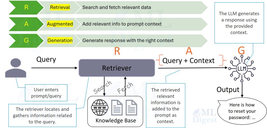
Imagine a research assistant standing in a library. A standard retrieval-augmented generation (RAG) system gives that assistant a stack of pages that look similar to the question. A knowledge-graph-based retrieval-augmented generation (KG-RAG) system gives the assistant something more useful: the pages, the named entities inside them, and the explicit relationships that connect those entities. That extra structure is often the difference between finding similar text and following the chain of evidence needed to answer a multi-step question.
KG-RAG builds on the original RAG idea and extends it with a knowledge graph over entities, relations, chunks, or documents. Recent systems such as Microsoft Research’s GraphRAG have shown why this matters in practice: many difficult questions are not only about semantic similarity, they are about connecting facts across multiple sources.
This article explains why KG-RAG matters, how the system works, the mathematics behind graph-aware retrieval, how to build one step by step, and how to implement a small but runnable prototype in Python.
1. Why Knowledge-Graph-Based RAG Matters
Plain RAG is very strong when the answer sits inside one or two chunks that are semantically similar to the query. It starts to struggle when the question has one of these properties:
- It requires multi-hop reasoning across several documents.
- It mentions entities that have aliases, abbreviations, or indirect references.
- It asks for relationships rather than isolated facts.
- It needs controllable provenance, such as “which document supports this connection?”
- It benefits from traversing a neighborhood of related facts instead of retrieving only by vector similarity.
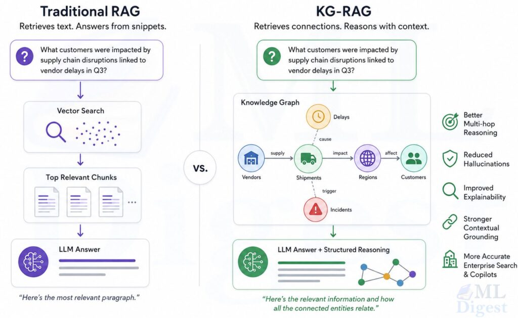
Consider the question: “Which retrieval method is commonly paired with a graph database in enterprise RAG pipelines, and why is that combination useful for compliance questions?”
A dense retriever may find chunks about graph databases and separate chunks about lexical retrieval. A knowledge graph can explicitly connect concepts such as “Neo4j”, “BM25“, “entity-centric retrieval”, and “provenance”, then expand from those anchors before the generator writes the answer.
The core benefit is simple: a graph turns hidden structure into retrievable structure.
What a knowledge graph contributes
A knowledge graph usually stores some combination of:
- Entities, such as people, companies, models, datasets, and products.
- Relations, such as “works on”, “depends on”, “acquired”, or “evaluated on”.
- Source references, so each edge can point back to evidence.
- Optional higher-level structure, such as communities, topics, or document hierarchies.
Once that structure exists, retrieval can do more than nearest-neighbor search. It can start from seed entities in the query, walk to related nodes, prioritize supporting subgraphs, and then package a context window that preserves relationships instead of flattening everything into disconnected chunks.
Grapg-based RAG are not useful; sometimes vanilla RAG wins. Follow this post for additional info.
2. Core System Architecture
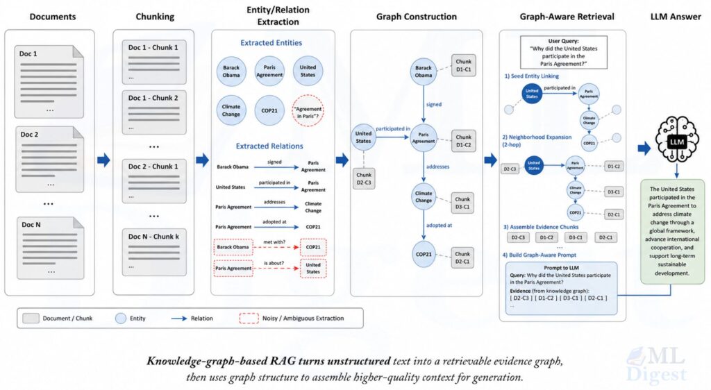
A practical KG-RAG system usually has six stages: ingestion, entity and relation extraction, graph construction, query understanding and graph seeding, graph-aware retrieval, and context assembly with answer generation.
2.1 Ingestion and Chunking
You still begin with raw documents, PDFs, web pages, tickets, or database exports. These are usually split into chunks before indexing.
Chunking matters because the graph is only as good as the evidence attached to it.
Good chunking guidelines:
- Keep chunks small enough to stay focused, usually 200 to 600 tokens for many document collections.
- Preserve local coherence, such as section boundaries, tables, or bullet groups.
- Store document metadata, timestamps, authors, and access controls with every chunk.
In a graph-oriented system, each chunk often becomes a first-class object because it is the evidence unit that later supports retrieved entities and relations.
2.2 Entity and Relation Extraction
Next, the system extracts structured information from chunks. This can be done with spaCy pipelines, rule-based matchers, supervised information extraction models, or large language model (LLM)-based extraction prompts.
Typical outputs include:
- Named entities: “Neo4j”, “BM25”, “FDA”, “Transformer”
- Relation triples: $(h, r, t)$ such as $(\text{GraphRAG}, \text{builds}, \text{community summaries})$
- Claims or events with timestamps
- Canonical IDs after entity resolution, for example mapping “MSFT” and “Microsoft” to the same node
This stage is where many systems either become reliable or become noisy. If the extractor invents relations, the graph will faithfully preserve those mistakes.
2.3 Graph Construction
The graph can be modeled in several ways.
- A document-entity bipartite graph.
Documents or chunks connect to the entities they mention. - An entity-relation graph.
Entities connect directly through typed edges. - A hybrid graph.
Documents, chunks, entities, relations, communities, and summaries all become nodes.
In practice, hybrid graphs are common because they support both evidence retrieval and abstract reasoning.
Useful node types: chunk, document, entity, claim, event, community, summary.
Useful edge types: MENTIONS, MENTIONED_IN, RELATED_TO, EVALUATED_ON, WORKS_ON, DEPENDS_ON, ACQUIRED, PART_OF, CAUSES, COMPARE_TO, SIMILAR_TO, MENTIONED_WITH, MENTIONED_NEAR, MENTIONED_IN_SAME_DOCUMENT.
2.4 Query Understanding and Graph Seeding
Before the system can search the graph, it needs to understand what the user is actually asking. This stage is called query understanding, and it answers a simple question: “Which parts of this question should we use as entry points into the graph?”
Think of it like arriving at a library and telling the librarian your topic. The librarian does not start reading every book. Instead, they first identify the key concepts in your question, then walk directly to the relevant shelves. Query understanding is that first step: identifying the key concepts before any retrieval happens.
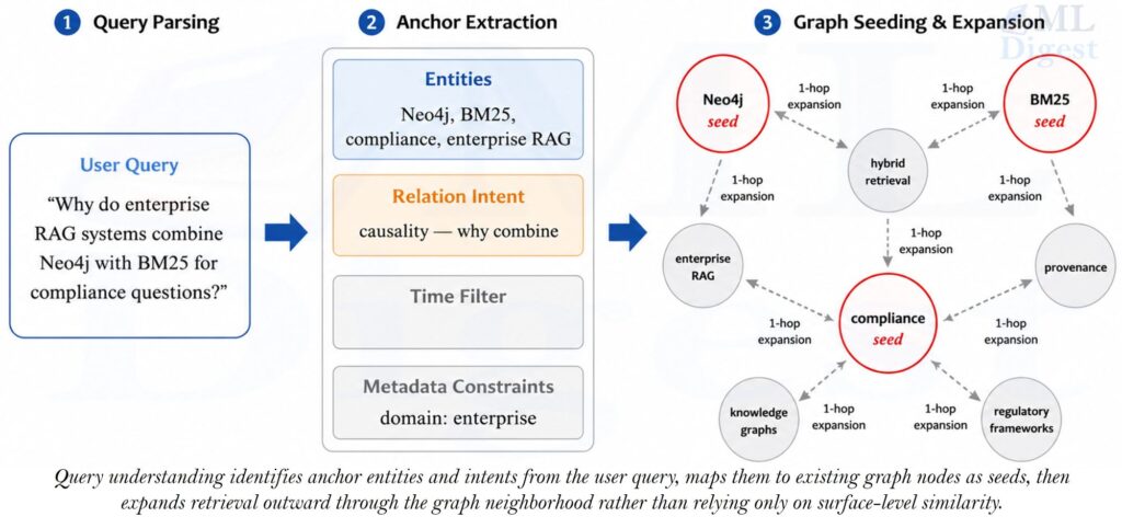
The system parses the query into pieces called anchors. An anchor is any part of the question that can be matched to a node already in the graph. These anchors may include:
- entities mentioned explicitly in the query — names of people, products, companies, models, or concepts that appear as nodes in the graph (for example “Neo4j” or “BM25”)
- relation intents — the kind of connection the user is asking about, such as comparison (“which is better”), causality (“why does X cause Y”), or dependency (“what does X rely on”)
- time filters — date ranges or relative time expressions such as “last quarter” or “before 2023”
- metadata constraints — structural filters such as department, author, document type, or access region
For example, consider the query: “Why do enterprise RAG systems combine Neo4j with BM25 for compliance questions?”
The anchors extracted from this query would be:
- entities:
Neo4j,BM25,enterprise RAG,compliance - relation intent: causality (“why … combine”)
These anchors are then matched to nodes that already exist in the graph. The matched nodes become the starting points for graph traversal. This step is called graph seeding.
Graph seeding matters because the graph can be large. Without a starting point, traversal would have to explore everything. With seeds, the system starts exactly where the question points and expands outward from there, following edges to nearby evidence. The quality of the seeds directly determines whether the traversal finds the right evidence or drifts into unrelated neighborhoods.
2.5 Graph-Aware Retrieval
This is the heart of the system, and the step that most clearly separates KG-RAG from plain RAG.
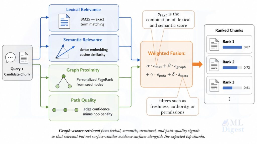
In practice, the retriever does not rely on a single relevance score. It combines several signals at once.
Lexical relevance checks whether the words in a chunk literally match the words in the query. This is often measured with BM25, a ranking function that rewards chunks containing the exact terms from the question, weighted by how rare those terms are across the corpus. This signal is especially important when the query contains identifiers, policy language, or precise technical terms where paraphrase detection would miss the point.
Semantic relevance checks whether the meaning of a chunk matches the meaning of the query, even if the words are different. This is measured using dense embeddings: the query and each chunk are encoded as vectors, and chunks whose vectors point in a similar direction are ranked higher. A chunk about “car engine failure” would score well for the query “automobile breakdown” even if neither phrase appears in the other.
Graph proximity is the new ingredient. Once the query has been seeded with anchor entities (from section 2.4), the retriever scores each chunk by how close it sits to those anchors in the graph. A chunk that directly mentions a seeded entity receives a high proximity score. A chunk connected to a seeded entity by two or three hops receives a lower but still meaningful score. This is how the system finds evidence that does not look similar to the query on the surface but is structurally related to it through shared entities.
Path quality rewards chunks that are reachable through short, well-supported relation chains rather than long, speculative ones. A direct edge between two high-confidence entities scores better than a five-hop path through loosely related nodes. This discourages the system from retrieving tangentially connected evidence just because the graph can technically reach it.
Metadata filters and permissions ensure that structural relevance does not override access rules or freshness requirements. A chunk that is graph-adjacent but belongs to a restricted team, or one that is highly ranked but two years stale, should be filtered or penalized before it enters the context window.
These signals are combined into a single ranked list, typically as a weighted sum as described in section 3.1. Instead of asking only “which chunk looks similar to the query?”, the retriever asks “which chunks, entities, and paths are both relevant and structurally supportive?”
A useful way to remember the difference: lexical and semantic signals tell you what a chunk is about, while graph proximity and path quality tell you where that chunk sits in the web of evidence. Both dimensions together produce a much more reliable shortlist than either alone.
2.6 Context Assembly and Answer Generation
Once the system has candidate nodes and chunks, it needs to build a prompt.
This often includes:
- the top evidence chunks
- extracted triples or path summaries
- document titles and timestamps
- short graph-derived explanations, such as “A connects to B through C”
The generator then produces the answer while citing the retrieved evidence. Strong systems keep the graph itself out of the final prose unless it helps explain the answer. The goal is not to show the graph, the goal is to use the graph to improve retrieval, faithfulness, and traceability.
3. The Mathematical View
The cleanest way to think about KG-RAG is as a ranking problem over structured evidence.
3.1 Hybrid Retrieval Score
Let $q$ be the user query and $d$ be a candidate chunk or document. A common ranking form is:
$$
s(d \mid q) = \alpha s_{\text{text}}(q, d) + \beta s_{\text{graph}}(q, d) + \gamma s_{\text{path}}(q, d) + \delta s_{\text{meta}}(q, d)
$$
where:
- $s_{\text{text}}$ is a lexical or embedding-based relevance score
- $s_{\text{graph}}$ measures how close $d$ is to query-seeded graph nodes
- $s_{\text{path}}$ rewards high-quality reasoning paths or relation chains
- $s_{\text{meta}}$ incorporates filters such as freshness, authority, or permissions
- $\alpha, \beta, \gamma, \delta$ are tunable weights
This form is practical because it reflects how real systems work. They fuse several weakly correlated signals instead of hoping one retriever handles every query type.
3.2 Graph Proximity with Personalized PageRank
One useful way to score graph relevance is Personalized PageRank, which scores how relevant each node in a graph is to a set of query seed nodes by running a random walk that occasionally restarts at those seeds. Suppose the graph has transition matrix $P$ and a restart vector $e_q$ concentrated on query seed nodes. Then the stationary relevance vector $\pi_q$ satisfies:
$$
\pi_q = (1 – \lambda)e_q + \lambda P^\top \pi_q
$$
where $\lambda \in [0, 1)$ is the walk continuation probability.
The equation balances two forces: the walk explores the graph structure (with probability $\lambda$), but it also keeps returning to the query seeds (with probability $1 – \lambda$). Nodes that are close to the seeds and well-connected receive higher scores.
Intuition:
- The walk repeatedly returns to query anchors.
- Nodes close to those anchors receive more probability mass.
- Documents connected to important entities become stronger candidates.
If a document node $d$ has large $\pi_q(d)$, then it lies in a graph neighborhood that is strongly related to the query anchors.
3.3 Path-Based Evidence Scoring
For multi-hop questions, it is useful to score not only nodes but also paths. If $p = (v_0, v_1, \dots, v_k)$ is a path from a seeded entity to a candidate evidence node, a simple scoring form is:
$$
s_{\text{path}}(p) = \sum_{i=1}^{k} w(v_{i-1}, v_i) – \eta k
$$
where $w(v_{i-1}, v_i)$ is the confidence or importance of each edge and $\eta$ penalizes long paths.
This captures an important trade-off: long chains may connect more concepts, but they also increase the risk of drifting away from the true answer.
3.4 Context Packing as a Constrained Optimization Problem
After retrieval, the system still needs to fit evidence into a limited context window. If each candidate chunk $d_i$ has token cost $c_i$ and utility $u_i$, context packing resembles a knapsack problem:
$$
\max_{x_i \in {0,1}} \sum_i u_i x_i \quad \text{subject to} \quad \sum_i c_i x_i \le B
$$
where $B$ is the token budget.
In practice, the utility $u_i$ often includes diversity penalties so the prompt does not waste tokens on five chunks that say the same thing.
3.5 Why the Math Matters
These formulations are not merely academic. They identify precisely where system quality comes from:
- better seed extraction improves $e_q$
- better graph edges improve $P$
- better confidence calibration improves edge weights $w$
- better prompt packing improves the final utility under a fixed budget
If any one of these parts is poor, the graph can become an expensive distraction rather than a real retrieval advantage.
4. How to Build a Knowledge-Graph-Based RAG System
This section gives a practical implementation blueprint.
4.1 Step 1: Define the Graph Schema Before Indexing
Many teams start by extracting triples immediately. This is often counterproductive. First define what the graph must support.
Ask these questions:
- Do you need evidence at the chunk level or only the document level?
- Will users ask relation questions, summarization questions, or global trend questions?
- Do you need typed edges, temporal edges, or source-aware edges?
- Do you need row-level access control?
If you do not define the schema first, you often end up with a graph that is hard to query and expensive to maintain.
4.2 Step 2: Build a Reliable Extraction Pipeline
At minimum, store:
- the raw chunk text
- extracted entities
- normalized entity IDs
- extracted relations with confidence scores
- evidence spans or source chunk IDs
Best practice is to separate extraction confidence from graph existence. An edge should carry metadata such as source, model version, extraction timestamp, and confidence score.
4.3 Step 3: Choose the Right Storage Layer
For local prototyping, NetworkX is excellent. For production graph queries, graph databases such as Neo4j are a common choice. Most production systems also keep a vector index alongside the graph, built with libraries such as FAISS or managed stores such as Chroma, together with a metadata store.
This means a real architecture often has three storage views:
- a document or chunk store
- a vector index
- a graph store
That split is normal. The graph does not replace everything else.
4.4 Step 4: Implement Query-Time Fusion
A reliable retrieval routine usually does the following:
- Parse the query into entities, intents, filters, and keywords.
- Retrieve initial candidates with lexical or dense search.
- Seed the graph with detected entities or top retrieved chunks.
- Expand a bounded neighborhood or run Personalized PageRank.
- Re-rank candidates with a fused score.
- Pack supporting evidence into the prompt.
This staged design is much easier to debug than a monolithic “one retriever does everything” system.
4.5 Step 5: Generate Answers with Explicit Provenance
Each answer should be backed by evidence references. Good answer objects usually store:
- cited chunk IDs
- cited relation paths
- confidence or answerability signals
- unresolved ambiguities
If the system cannot find a coherent path or enough evidence, the answer should say that explicitly.
5. A Runnable Python Prototype
The following example is deliberately small. It uses scikit-learn for lexical similarity and networkx for graph scoring. The entity extraction is rule-based so that the example stays runnable without external APIs. In a production system, you would usually replace the entity extractor with a stronger information extraction pipeline and replace TF-IDF with dense retrieval.
from itertools import combinations
import re

import networkx as nx
import numpy as np
from sklearn.feature_extraction.text import TfidfVectorizer
from sklearn.metrics.pairwise import cosine_similarity


DOCUMENTS = [
    {
        "id": "doc_1",
        "text": (
            "GraphRAG extracts entities, relations, and claims from source documents "
            "before building a graph that supports local search and community summaries."
        ),
    },
    {
        "id": "doc_2",
        "text": (
            "Neo4j is often used as a graph database in enterprise RAG systems because "
            "it stores nodes, edges, properties, and provenance in a queryable structure."
        ),
    },
    {
        "id": "doc_3",
        "text": (
            "BM25 remains useful in RAG because compliance and audit questions often "
            "depend on exact terms, identifiers, and policy language."
        ),
    },
    {
        "id": "doc_4",
        "text": (
            "Hybrid retrieval combines lexical ranking with semantic retrieval so that "
            "systems can preserve exact matches while still capturing paraphrases."
            "Neo4j's graph structure complements hybrid retrieval by connecting related concepts that may not be lexically similar."
        ),
    },
    {
        "id": "doc_5",
        "text": (
            "Knowledge graphs help multi-hop retrieval because they make relationships "
            "between entities explicit and traversable."
            "GraphRAG builds community summaries to support global search across graph neighborhoods."
        ),
    },
]

ENTITY_CATALOG = [
    "graphrag",
    "neo4j",
    "bm25",
    "enterprise rag",
    "compliance",
    "audit",
    "hybrid retrieval",
    "semantic retrieval",
    "knowledge graphs",
    "multi-hop retrieval",
    "community summaries",
    "provenance",
]


def normalize_text(text: str) -> str:
    return re.sub(r"\s+", " ", text.lower()).strip()


def extract_entities(text: str, entity_catalog: list[str]) -> list[str]:
    normalized = normalize_text(text)
    matches = [entity for entity in entity_catalog if entity in normalized]
    return sorted(set(matches))


def min_max_scale(values: np.ndarray) -> np.ndarray:
    values = np.asarray(values, dtype=float)
    if np.allclose(values.max(), values.min()):
        return np.zeros_like(values)
    return (values - values.min()) / (values.max() - values.min())


def build_graph(documents: list[dict], entity_catalog: list[str]):
    graph = nx.Graph()
    doc_entities = {}

    for document in documents:
        doc_id = document["id"]
        graph.add_node(doc_id, kind="document", text=document["text"])

        entities = extract_entities(document["text"], entity_catalog)
        doc_entities[doc_id] = entities

        for entity in entities:
            graph.add_node(entity, kind="entity")
            graph.add_edge(doc_id, entity, relation="MENTIONS", weight=1.0)

        for left, right in combinations(entities, 2):
            if graph.has_edge(left, right):
                graph[left][right]["weight"] += 1.0
            else:
                graph.add_edge(left, right, relation="CO_OCCURS_WITH", weight=1.0)

    return graph, doc_entities


def build_text_index(documents: list[dict]):
    vectorizer = TfidfVectorizer(stop_words="english")
    matrix = vectorizer.fit_transform([document["text"] for document in documents])
    return vectorizer, matrix


def seed_personalization(query: str, graph: nx.Graph, entity_catalog: list[str]) -> tuple[list[str], dict]:
    seeds = extract_entities(query, entity_catalog)
    personalization = {node: 0.0 for node in graph.nodes}

    for seed in seeds:
        if seed in personalization:
            personalization[seed] = 1.0

    return seeds, personalization


def explain_document(doc_id: str, doc_entities: dict, seeds: list[str]) -> str:
    entities = doc_entities.get(doc_id, [])
    overlap = [entity for entity in entities if entity in seeds]
    if overlap:
        return f"matched query entities: {', '.join(overlap)}"
    if entities:
        return f"related entities in graph: {', '.join(entities[:3])}"
    return "selected primarily by text similarity"


def rank_documents(query: str, documents: list[dict], graph: nx.Graph, doc_entities: dict, vectorizer, matrix):
    query_vector = vectorizer.transform([query])
    lexical_scores = cosine_similarity(query_vector, matrix)[0]

    seeds, personalization = seed_personalization(query, graph, ENTITY_CATALOG)
    if sum(personalization.values()) == 0.0:
        best_doc = documents[int(np.argmax(lexical_scores))]["id"]
        personalization[best_doc] = 1.0

    pagerank_scores = nx.pagerank(graph, alpha=0.85, personalization=personalization, weight="weight")
    graph_scores = np.array([pagerank_scores[document["id"]] for document in documents])

    lexical_scores = min_max_scale(lexical_scores)
    graph_scores = min_max_scale(graph_scores)
    final_scores = 0.65 * lexical_scores + 0.35 * graph_scores

    ranked = []
    for document, lexical_score, graph_score, final_score in zip(
        documents, lexical_scores, graph_scores, final_scores
    ):
        ranked.append(
            {
                "id": document["id"],
                "text": document["text"],
                "lexical": round(float(lexical_score), 3),
                "graph": round(float(graph_score), 3),
                "final": round(float(final_score), 3),
                "why": explain_document(document["id"], doc_entities, seeds),
            }
        )

    ranked.sort(key=lambda item: item["final"], reverse=True)
    return seeds, ranked


if __name__ == "__main__":
    graph, doc_entities = build_graph(DOCUMENTS, ENTITY_CATALOG)
    vectorizer, matrix = build_text_index(DOCUMENTS)

    query = "Why do enterprise RAG systems combine Neo4j with BM25 for compliance questions?"
    seeds, ranked = rank_documents(query, DOCUMENTS, graph, doc_entities, vectorizer, matrix)

    print("Seed entities:", seeds)
    print()
    for item in ranked[:3]:
        print(item["id"], item["final"], item["why"])
        print("  text:", item["text"])
        print("  lexical:", item["lexical"], "graph:", item["graph"])
print()Some of the relation triples in the graph are:
(doc_1, MENTIONS, community summaries)
(doc_1, MENTIONS, graphrag)
(community summaries, CO_OCCURS_WITH, graphrag)
(community summaries, MENTIONS, doc_5)
(community summaries, CO_OCCURS_WITH, knowledge graphs)
(community summaries, CO_OCCURS_WITH, multi-hop retrieval)
(graphrag, MENTIONS, doc_5)
(graphrag, CO_OCCURS_WITH, knowledge graphs)
(graphrag, CO_OCCURS_WITH, multi-hop retrieval)
(doc_2, MENTIONS, enterprise rag)
(doc_2, MENTIONS, neo4j)
(doc_2, MENTIONS, provenance)
(enterprise rag, CO_OCCURS_WITH, neo4j)
(enterprise rag, CO_OCCURS_WITH, provenance)
...
...
(neo4j, CO_OCCURS_WITH, provenance)
(neo4j, MENTIONS, doc_4)
(neo4j, CO_OCCURS_WITH, hybrid retrieval)
5.1 What This Example Demonstrates
This prototype shows the essential KG-RAG loop:
- Index documents as both text and graph structure.
- Detect entity anchors in the query.
- Use those anchors to seed a graph score.
- Fuse graph evidence with text relevance.
- Return evidence with an explanation.
The implementation is intentionally simple, but the design pattern scales.
5.2 How to Make the Prototype Production-Ready
The next upgrades are usually:
- replace rule-based entity matching with a proper extraction and entity-linking pipeline
- replace TF-IDF with dense retrieval or hybrid retrieval
- store graph edges with provenance and confidence
- add metadata filters and access control
- introduce reranking before prompt assembly
- cache popular graph neighborhoods for latency control
Frameworks such as LangChain and LlamaIndex provide pre-built integrations for several of these stages, including graph store connectors, hybrid retrieval pipelines, and reranking components, which can reduce implementation effort considerably.
6. Practical Design Choices
6.1 Choose the Right Graph Granularity
There is no single correct graph design.
- If you need factual precision, connect chunks to entities and store evidence spans.
- If you need broad summarization, add community or topic nodes.
- If you need process reasoning, model events and timestamps explicitly.
The question type should determine the graph granularity.
6.2 Control Graph Expansion Carefully
Unbounded traversal is a common failure mode. A graph can connect almost anything if you let it walk far enough.
Useful controls include:
- maximum hop count
- minimum edge confidence
- relation type filters
- node type filters
- temporal constraints
Without these constraints, retrieval quality often drops because the system over-expands into loosely related neighborhoods.
6.3 Keep Provenance Attached to Every Fact
This is one of the biggest practical wins of KG-RAG. Every useful edge should remember:
- source document or chunk ID
- extraction method or model version
- extraction timestamp
- confidence score
- optional human validation status
If an answer cites a relation but you cannot trace it back to source text, the graph is not doing enough for governance or debugging. In regulated environments, this provenance trail also pairs naturally with LLM guardrails to block or flag answers that lack verified source evidence.
6.4 Combine Graph Retrieval with Classic Retrieval
One of the biggest mistakes is treating graph retrieval as a total replacement for lexical or dense retrieval.
In practice:
- lexical search is excellent for exact identifiers and policy wording
- dense search is strong for paraphrases and semantic similarity
- graph retrieval is strong for entity-centric navigation and multi-hop expansion
The best systems usually combine all three.
6.5 Decide Whether You Need Local Search or Global Search
Some questions ask for a specific grounded answer. Others ask for a high-level synthesis across a large corpus.
- Local search starts from seeded entities and finds nearby evidence.
- Global search aggregates over graph communities or summaries to answer broad questions.
This distinction is one reason GraphRAG-style systems often build community summaries in addition to local entity graphs.
7. Common Failure Modes
7.1 Noisy Extraction Creates a Noisy Graph
If relation extraction is weak, the graph becomes a high-confidence storage layer for low-confidence facts. This can hurt retrieval more than it helps it. A common mitigation is to attach confidence scores to every extracted edge and filter out low-confidence relations at query time rather than at indexing time. That way the raw graph preserves all evidence, but retrieval only walks edges that meet a minimum quality threshold.
7.2 Entity Resolution Is Harder Than It Looks
“Apple” the company, “apple” the fruit, and internal product codenames are not rare corner cases. If entity linking is poor, graph traversal starts from the wrong node. Abbreviations, acronyms, and name variants compound the problem: “MSFT”, “Microsoft Corp.”, and “Microsoft” may all appear in the same corpus. Without a dedicated resolution step that maps surface forms to canonical IDs, the graph fragments into disconnected clusters that should have been one connected component.
7.3 Path Quality Can Look Convincing While Being Wrong
Graphs are excellent at producing plausible connection chains. That does not mean each edge is valid. This is why source-backed edges and confidence weighting matter.
7.4 Prompt Packing Can Erase Graph Benefits
Even if retrieval finds the right subgraph, a poor prompt packer can flatten it into an incoherent context window. For example, if the packer simply concatenates chunks in arbitrary order, the generator may not see which entities are connected or which chunk supports which relation. Good context assembly preserves both evidence and relation structure, for instance by grouping chunks around their shared entities or by including short relation summaries between evidence blocks.
7.5 Latency Can Grow Quickly
A production KG-RAG pipeline may include extraction, entity linking, vector retrieval, graph traversal, reranking, and generation. If you do not budget latency early, the system becomes difficult to operate. Common mitigations include caching frequently accessed graph neighborhoods, pre-computing Personalized PageRank vectors for common entity seeds, limiting traversal depth to a conservative default, and using approximate nearest-neighbor search instead of exact search for the vector retrieval step.
8. Best Practices
- Start with a narrow domain where the entity vocabulary is reasonably stable. A focused domain, such as a single product line, a regulatory corpus, or an internal knowledge base, gives the extraction pipeline a realistic chance of producing clean entities. Expanding to broader domains can come after the core pipeline proves itself.
- Measure gains on the right queries. Evaluate on multi-hop and provenance-sensitive questions, not only on easy semantic similarity queries. General guidance on measuring LLM performance covers complementary metrics such as faithfulness and answer relevance that apply directly to KG-RAG outputs. Standard benchmarks such as HotpotQA and MuSiQue cover multi-hop reasoning, while provenance-focused evaluation may require domain-specific test sets. If the benchmark consists entirely of single-hop lookups, the graph will appear to add cost without benefit.
- Keep a plain RAG baseline so you can prove the graph is actually helping. Without a controlled comparison, it is easy to attribute improvements to the graph when they really come from better chunking, improved prompts, or other pipeline changes.
- Store source evidence with every extracted fact. Every triple or relation in the graph should trace back to at least one chunk and its originating document. This supports debugging, auditability, and user trust.
- Make graph expansion bounded and observable. Set explicit limits on hop count, maximum neighborhood size, and minimum edge confidence. Log the expansion path for every query so that retrieval behavior can be inspected after the fact.
- Audit entity resolution errors early. Duplicate or mislinked entities create downstream retrieval failures that are hard to diagnose because the symptoms appear in answer quality, not in the extraction logs. Periodic spot checks on the entity table catch these problems before they compound.
- Log which seed entities, paths, and chunks were used for each answer. This retrieval trace is essential for debugging poor answers and for understanding whether the graph is contributing meaningfully to retrieval or simply adding latency.
When KG-RAG Is the Right Tool
KG-RAG is especially useful when:
- the corpus has repeated entities across many documents
- users ask relationship-heavy or multi-hop questions
- provenance, compliance, or investigation workflows matter
- the domain already has structured concepts, such as customers, products, contracts, or incidents
It is less useful when the corpus is small, the questions are shallow, or relation extraction quality is poor. In those cases, a strong hybrid RAG pipeline without a graph may be simpler and more reliable.
Summary
KG-RAG improves standard RAG by making entities and relationships explicit, retrievable, and traceable. The main idea is straightforward: combine text retrieval with graph-aware reasoning so the system can follow evidence paths instead of relying only on chunk similarity. The real engineering work lies in reliable extraction, careful graph design, bounded traversal, and prompt assembly that preserves provenance.
If you want to apply this in practice, start with a narrow domain, build a small hybrid prototype, and compare it against a strong non-graph baseline on multi-hop and compliance-style questions. That experiment will tell you quickly whether the graph is adding real retrieval signal or only architectural complexity.

Happy is a seasoned ML professional with over 15 years of experience. His expertise spans various domains, including Computer Vision, Natural Language Processing (NLP), and Time Series analysis. He holds a PhD in Machine Learning from IIT Kharagpur and has furthered his research with postdoctoral experience at INRIA-Sophia Antipolis, France. Happy has a proven track record of delivering impactful ML solutions to clients.

Silpa brings 5 years of experience in working on diverse ML projects, specializing in designing end-to-end ML systems tailored for real-time applications. Her background in statistics (Bachelor of Technology) provides a strong foundation for her work in the field. Silpa is also the driving force behind the development of the content you find on this site.
Subscribe to our newsletter!