Imagine a model that predicts loan defaults. During training, the pipeline pulls account_balance from the warehouse today, but the examples come from loans scored a year ago. For defaulted loans, today’s balance reflects post-default reality: accounts may be closed, sent to collections, or restructured. The model quietly learns to recognize the financial footprint left behind by default. At scoring time, none of that has happened yet. Offline accuracy looks excellent, online performance collapses, and the root cause is not the model. It is the timeline.
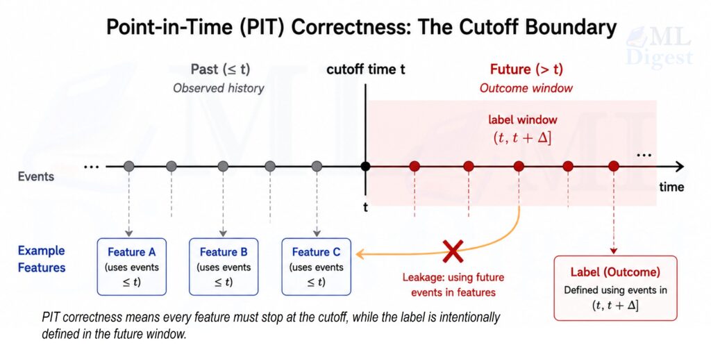
Point-in-time correctness, usually shortened to PIT correctness, is the discipline of ensuring that every feature in a training row could truly have been known when the prediction was supposed to happen. This class of problem is also commonly called temporal leakage. The model may read the past. The label may look into the future. The boundary between them must be explicit, testable, and enforced.
This is one of the most common ways ML systems accidentally leak information. The leakage often looks harmless because it hides inside routine joins, snapshots, rolling windows, and status columns. The goal of PIT correctness is to turn that vague risk into a concrete data contract.
1. Why PIT correctness matters
Suppose you are predicting whether a customer will churn in the next 7 days. At scoring time on Monday at 9:00 AM, the model should only see information that was already available by Monday at 9:00 AM. If the training set accidentally includes a support ticket created on Tuesday, or a status field updated after the customer already started cancellation, the model is learning from a future that production will never see.
That is the heart of PIT correctness: each training example must reconstruct the information boundary that existed at prediction time.
When teams get this wrong, the symptoms are familiar:
- validation metrics look suspiciously strong
- online performance drops after deployment
- training and serving feature distributions diverge
- small ingestion delays create surprisingly large performance regressions
PIT correctness matters because it makes offline evaluation trustworthy. It also reduces training-serving skew, makes incidents easier to debug, and forces the team to describe data semantics precisely enough to survive backfills, late arrivals, and pipeline rewrites.
2. The core contract
The cleanest way to reason about PIT correctness is to define every training row as an entity-time pair.
For each observation, specify:
- entity $e$, such as a user, account, device, listing, or merchant
- cutoff time $t$, also called as-of time or observation time
- label horizon $\Delta$, such as the next 7 days or next 30 days
Once those three pieces are explicit, PIT correctness reduces to two rules.
2.1 Feature rule
Every feature at $(e, t)$ must be a function of information available at or before $t$:
$$
\mathbf{x}(e, t) = f\big(e, \mathcal{I}(t)\big).
$$
Operationally, this means:
- joins must not pull rows from after $t$
- rolling windows must end at $t$
- latest-known-value lookups must use an as-of join
- tie-breaking rules must be deterministic
2.2 Label rule
The label must be defined in a future interval relative to $t$. A common choice is:
$$
y(e, t) = \mathbb{1}{\text{event occurs in } (t, t + \Delta]}.
$$
Labels intentionally come from the future. Features must not touch that future.
2.3 Boundary conventions
Most real leakage bugs live in small ambiguities, not dramatic failures. Boundary rules should therefore be written down once and reused everywhere.
One safe convention is:
- features include rows with
event_time <= t - labels include rows with
event_time > t AND event_time <= t + Delta
If you work at day granularity, you also need to define what counts as the end of day and keep that definition identical in training and serving. Timezone handling matters here: if cutoff timestamps are stored in UTC but source tables write event times in local time, the boundary can silently shift by several hours, producing hard-to-trace leakage.
3. Two notions of time: event time and availability time
Many PIT explanations sound correct while still hiding one unresolved question: available according to which clock?
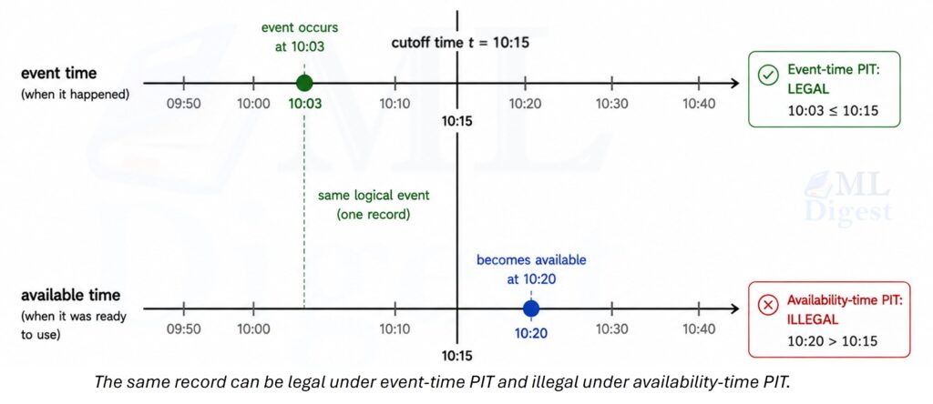
3.1 Event-time PIT
Under event-time PIT, a fact is considered usable if it happened by time $t$. This gives the cleanest historical reconstruction of the world and is often useful for research and diagnosis.
Example: a purchase happened at 10:03 AM but landed in the warehouse at 10:20 AM. Under event-time PIT, that purchase belongs to a cutoff at 10:15 AM because it truly happened before the cutoff.
3.2 Availability-time PIT
Under availability-time PIT, a fact is usable only if the system could actually have served it by time $t$. This is usually the better choice for production-bound evaluation because it captures ingestion lag, freshness guarantees, and feature pipeline latency.
In mature datasets, it is common to keep both:
event_time, when the underlying event happenedavailable_time, when the feature pipeline could legally use the event
3.3 Which one should you use?
Use event-time PIT when the goal is scientific diagnosis, signal discovery, or historical understanding.
Use availability-time PIT when the goal is deployment realism.
If storage and pipeline overhead allow, keep both. A practical pattern is:
- use an event-time dataset for research and failure analysis
- use an availability-time dataset for final offline evaluation before launch
4. Where leakage usually sneaks in
PIT problems are rarely dramatic. Most of them look like ordinary joins, ordinary aggregates, or ordinary status columns.
4.1 Window boundaries that drift past the cutoff
An aggregate such as purchases_last_30d sounds harmless. But if the implementation quietly scans through the end of the current partition rather than the true cutoff, the feature is no longer PIT-safe.
Common causes include:
- using partition-level day boundaries instead of the exact cutoff timestamp
- including same-day events that happened after the cutoff
- using
now()in feature code that should be using the row-specificas_of_time
4.2 Latest-state joins without an as-of condition
A table that stores account_status, risk_tier, or current_plan is often updated over time. If you join the latest row without checking whether it existed before $t$, you have leaked the future in a single line of SQL.
4.3 Outcome proxies
Sometimes the label itself is not joined directly, but a proxy is just as revealing.
Examples:
- predicting chargeback while using
dispute_opened_flag - predicting churn while using
account_closed_timestamp - predicting suspension while using
suspension_reason
These fields may be valid warehouse columns, but they are not valid model inputs for earlier cutoff times. They are typically populated as part of the same workflow that produces the outcome, which means they carry signal only because the outcome has already happened. At scoring time, that signal does not exist. Outcome proxy leakage is especially common in real-time fraud detection systems, where dispute and chargeback flags are tightly coupled to the outcome being predicted.
4.4 Retrospectively corrected tables
Daily snapshots and backfilled aggregates can become dangerous because they are often rewritten with cleaner knowledge than the production system had at the time. If you train on the corrected version without modeling when that correction became visible, you are training on a version of history that never existed online.
A common example is a daily transaction summary that is reprocessed each morning with prior-day adjustments applied. A training row with a Tuesday cutoff will silently read the Wednesday-corrected totals instead of the preliminary figures the production model would actually have seen on Tuesday.
5. Implementation blueprint
The implementation pattern is stable across warehouses, feature stores, and custom pipelines.
5.1 Build an observation spine first
Start with a table that defines the exact rows you want to train on. This is often called an observation spine.
Typical columns include:
entity_idas_of_time- optional cohort metadata
- optional label horizon metadata
This table matters because it gives every training row its own explicit clock. Without that clock, PIT correctness becomes hard to express and even harder to test.
5.2 Compute features relative to as_of_time
For each feature, answer one question: what data would have been legal at this row’s cutoff time?
This usually leads to one of two patterns.
Latest-known-value features
Examples include last known country, current plan, or most recent risk score.
Use an as-of join:
- join on entity keys
- filter rows with
source.event_time <= observation.as_of_time - if serving realism matters, also require
source.available_time <= observation.as_of_time
Window aggregate features
Examples include counts, sums, averages, and unique counts over the last 7, 30, or 90 days.
Use windows that end exactly at the cutoff:
$$
\text{window}(t, w) = (t – w, t].
$$
That means a safe event filter is typically event_time > window_start AND event_time <= as_of_time.
5.3 Compute labels separately
Do not let label logic leak into feature logic. Compute the label from raw future events in a separate step, then join it back only after features are complete.
That separation is one of the simplest ways to avoid accidental leakage through shared intermediate tables.
5.4 Validate before training
Before you fit a model, check that:
- every feature source has explicit time semantics
- boundary cases around the cutoff behave as intended
- obviously impossible columns are not present
- training and serving availability assumptions match
6. Worked SQL example
Suppose you want to predict whether an account will be suspended in the next 7 days. You train one row per account per day.
6.1 Observation spine
Your spine can be as simple as account_id, as_of_time.
The important part is not how elaborate the table looks. The important part is that every row carries an explicit cutoff.
6.2 PIT-safe feature examples
Assume you have these source tables:
logins(account_id, event_time, available_time, success)payments(account_id, event_time, available_time, status)account_country(account_id, event_time, available_time, country)
Window aggregate example
SELECT
    o.account_id,
    o.as_of_time,
    SUM(CASE WHEN l.success = TRUE THEN 1 ELSE 0 END) AS num_logins_7d
FROM observation_spine o
LEFT JOIN logins l
    ON l.account_id = o.account_id
   AND l.event_time > o.as_of_time - INTERVAL '7' DAY
   AND l.event_time <= o.as_of_time
   -- For serving realism, also require: AND l.available_time <= o.as_of_time
GROUP BY 1, 2;This feature is PIT-safe because the window is explicitly bounded by the observation time.
As-of join example
SELECT
    o.account_id,
    o.as_of_time,
    c.country AS last_country
FROM observation_spine o
LEFT JOIN (
    SELECT
        o2.account_id,
        o2.as_of_time,
        ac.country,
        ROW_NUMBER() OVER (
            PARTITION BY o2.account_id, o2.as_of_time
            ORDER BY ac.event_time DESC
        ) AS rn
    FROM observation_spine o2
    JOIN account_country ac
        ON ac.account_id = o2.account_id
       AND ac.event_time <= o2.as_of_time
       -- For serving realism, also require: AND ac.available_time <= o2.as_of_time
) c
    ON c.account_id = o.account_id
   AND c.as_of_time = o.as_of_time
AND c.rn = 1;This is the standard latest-known-value pattern. The predicate on event_time is the essential guardrail.
6.3 Label example
Assume you have suspensions(account_id, suspension_time).
Then the label for suspension in the next 7 days is:
SELECT
    o.account_id,
    o.as_of_time,
    CASE WHEN COUNT(s.suspension_time) > 0 THEN 1 ELSE 0 END AS suspended_next_7d
FROM observation_spine o
LEFT JOIN suspensions s
    ON s.account_id = o.account_id
   AND s.suspension_time > o.as_of_time
   AND s.suspension_time <= o.as_of_time + INTERVAL '7' DAY
GROUP BY 1, 2;6.4 What would leak in this example?
The following columns would be suspicious or outright illegal as features for earlier cutoff times:
suspension_reasonaccount_status = 'SUSPENDED'- a daily snapshot that was corrected later and does not preserve original availability semantics
7. Runnable Python example
The SQL patterns above show the production shape. The Python example below makes the time boundary visible line by line. It uses pandas only, so you can run it locally without a feature store.
7.1 What the code demonstrates
We will:
- create an observation spine
- build a window aggregate that respects the cutoff
- build a latest-known-value feature with an as-of join using pandas.merge_asof
- create a future label
- assert a few boundary conditions so the example behaves like a small PIT test
7.2 Code
import pandas as pd

# Observation spine: one row per entity-cutoff pair.
observation_spine = pd.DataFrame(
    {
        "account_id": [101, 101, 202],
        "as_of_time": pd.to_datetime(
            [
                "2025-01-10 12:00:00",
                "2025-01-15 12:00:00",
                "2025-01-10 12:00:00",
            ]
        ),
    }
).sort_values(["account_id", "as_of_time"])

# Atomic login events.
logins = pd.DataFrame(
    {
        "account_id": [101, 101, 101, 202],
        "event_time": pd.to_datetime(
            [
                "2025-01-05 10:00:00",
                "2025-01-10 11:59:59",
                "2025-01-10 12:00:01",  # Must be excluded for the first cutoff.
                "2025-01-08 09:00:00",
            ]
        ),
        "success": [True, True, True, True],
    }
)

# Slowly changing account attribute.
account_country = pd.DataFrame(
    {
        "account_id": [101, 101, 202],
        "event_time": pd.to_datetime(
            [
                "2025-01-01 00:00:00",
                "2025-01-12 00:00:00",
                "2025-01-02 00:00:00",
            ]
        ),
        "country": ["US", "CA", "FR"],
    }
).sort_values(["account_id", "event_time"])

# Future outcome events.
suspensions = pd.DataFrame(
    {
        "account_id": [101, 202],
        "suspension_time": pd.to_datetime(
            ["2025-01-16 08:00:00", "2025-01-25 08:00:00"]
        ),
    }
)

def add_num_logins_7d(spine: pd.DataFrame, login_events: pd.DataFrame) -> pd.DataFrame:
    rows = []
    for row in spine.itertuples(index=False):
        window_start = row.as_of_time - pd.Timedelta(days=7)
        mask = (
            (login_events["account_id"] == row.account_id)
            & (login_events["event_time"] > window_start)
            & (login_events["event_time"] <= row.as_of_time)
            & (login_events["success"])
        )
        rows.append(int(mask.sum()))

    result = spine.copy()
    result["num_logins_7d"] = rows
    return result

def add_last_country(spine: pd.DataFrame, country_events: pd.DataFrame) -> pd.DataFrame:
    merged = pd.merge_asof(
        spine.sort_values("as_of_time"),
        country_events.sort_values("event_time"),
        left_on="as_of_time",
        right_on="event_time",
        by="account_id",
        direction="backward",
        allow_exact_matches=True,
    )
    return merged[["account_id", "as_of_time", "country"]].rename(
        columns={"country": "last_country"}
    )


def add_label_suspended_next_7d(spine: pd.DataFrame, suspension_events: pd.DataFrame) -> pd.DataFrame:
    labels = []
    for row in spine.itertuples(index=False):
        mask = (
            (suspension_events["account_id"] == row.account_id)
            & (suspension_events["suspension_time"] > row.as_of_time)
            & (suspension_events["suspension_time"] <= row.as_of_time + pd.Timedelta(days=7))
        )
        labels.append(int(mask.any()))

    result = spine.copy()
    result["suspended_next_7d"] = labels
    return result


features = add_num_logins_7d(observation_spine, logins)
features = features.merge(
    add_last_country(observation_spine, account_country),
    on=["account_id", "as_of_time"],
    how="left",
)

dataset = features.merge(
    add_label_suspended_next_7d(observation_spine, suspensions),
    on=["account_id", "as_of_time"],
    how="left",
)

print(dataset.sort_values(["account_id", "as_of_time"]))

# Cheap PIT checks around the boundary.
first_row = dataset.sort_values(["account_id", "as_of_time"]).iloc[0]
assert first_row["num_logins_7d"] == 2, "Event after the cutoff leaked into the feature window."
assert first_row["last_country"] == "US", "The as-of join pulled a future country value."

# The later cutoff for account 101 should see the country change and the future suspension.
later_row = dataset.sort_values(["account_id", "as_of_time"]).iloc[1]
assert later_row["last_country"] == "CA"
assert later_row["suspended_next_7d"] == 1

print("All PIT checks passed.")7.3 What to notice in the code
The decisive details are small:
- the aggregate window ends at
as_of_time - the as-of join uses
direction="backward" - the label looks strictly after the cutoff
- the assertions exercise the boundary cases directly
In production, the same ideas often live in Feast, Tecton, or an internal feature platform. The tooling can change, but the semantics must not.
8. Validation, testing, and operating habits
PIT correctness is a data contract, so validation should be explicit and routine.
8.1 Start with boundary tests
Create tiny synthetic datasets with events at $t – 1$ second, exactly $t$, and $t + 1$ second. Then assert that features include only legal rows and labels start strictly after the cutoff. These tests catch a surprisingly large share of leakage bugs. Tools such as dbt data tests and Great Expectations can encode these boundary conditions as repeatable assertions that run automatically as part of the data pipeline. For a broader look at testing strategies across the ML development lifecycle, see Testing Machine Learning Code Like a Pro.
8.2 Add a few production smoke checks
If a feature suddenly looks too predictive, treat it as a data engineering incident until proven otherwise. Useful checks include:
- unusually high mutual information with the label
- columns that are populated offline but mostly missing online
- columns that only appear after the outcome workflow begins
- latency backtesting when availability times are recorded
- training-versus-serving comparisons for missingness, quantiles, category frequencies, and default-filled rates
If the distributions diverge immediately after launch, the cause is often a PIT or availability-time mismatch rather than concept drift.
8.3 Keep the contract visible in daily work
The habits are simple: carry as_of_time through every intermediate table, prefer atomic sources over corrected snapshots, version feature definitions when their semantics change, and use time-based evaluation when the problem is temporal. For many time series forecasting and risk settings, random splits hide the structure you are trying to preserve. TimeSeriesSplit in scikit-learn is a useful reference pattern.
9. A quick debugging checklist
If offline performance looks too good:
- check whether any join can pull rows with
event_time > as_of_time - check whether any aggregate window ends at
nowor partition end instead of the row cutoff - check whether a backfilled snapshot hides corrected future knowledge
- check whether a status field is really an outcome proxy
If online performance is much worse than offline:
- compare
event_timeandavailable_timesemantics - inspect online feature missingness and default values
- verify that the serving system applies the same boundary rules as training
Summary
Point-in-time correctness is the practice of making time explicit in ML data pipelines. Every training row needs a clearly defined cutoff time, every feature must stop at that boundary, and every label must start after it.
If you only remember three implementation moves, remember these:
- build an observation spine with
entity_idandas_of_time - compute features with explicit as-of joins and bounded windows
- compute labels separately in a future window
That small discipline prevents a large class of expensive failures. It also turns a vague warning about leakage into a concrete, testable contract.
If you want one final smell test for any training set, ask two questions:
- Could this exact feature row have been computed at scoring time?
- Would that still be true under normal data delays and late arrivals?
If either answer is unclear, the dataset is not ready yet.

Silpa brings 5 years of experience in working on diverse ML projects, specializing in designing end-to-end ML systems tailored for real-time applications. Her background in statistics (Bachelor of Technology) provides a strong foundation for her work in the field. Silpa is also the driving force behind the development of the content you find on this site.
Subscribe to our newsletter!