Multicollinearity in Linear Regression: Why Coefficients Become Unstable and How Ridge Regression Helps

When two or more features in a regression model are highly correlated, it becomes difficult to determine their individual impact. While the model may still predict well, the coefficients assigned to these features become unstable and sensitive to small changes in data.

This article explains why this instability occurs and how Ridge Regression provides a more stable solution by regularizing the model.

Why Multicollinearity Is a Problem

In ordinary least squares (OLS), the model tries to estimate a coefficient vector $\hat{\beta}$ that best fits the data:

$$
\hat{\beta}_{\text{OLS}} = (X^T X)^{-1} X^T y
$$

Here:

• $X$ is the design matrix
• $y$ is the target vector
• $\beta$ is the vector of true coefficients

When features are highly correlated, some columns of $X$ are close to being linear combinations of others. That makes $X^T X$ nearly singular, which means its inverse becomes numerically unstable. Once that happens, the coefficient estimates can swing dramatically even when the data changes only a little.

The practical consequence is important:

• Coefficients become unstable
• Standard errors become large
• Interpretation becomes unreliable
• Predictions may still look reasonable

That last point is what makes multicollinearity tricky. A model can appear to work while the coefficient values themselves are not trustworthy.

The Statistical View

Assume the usual linear model:

$$
y = X\beta + \varepsilon, \qquad \mathrm{Var}(\varepsilon) = \sigma^2 I
$$

Under these assumptions, the variance of the OLS estimator is:

$$
\mathrm{Var}(\hat{\beta}_{\text{OLS}}) = \sigma^2 (X^T X)^{-1}
$$

This equation is the core of the story. Multicollinearity shows up inside $(X^T X)^{-1}$. If $X^T X$ is close to singular, the entries of its inverse can become very large, and the variance of the coefficient estimates grows with them.

In other words:

$$
\text{multicollinearity} \Rightarrow X^T X \text{ nearly singular} \Rightarrow (X^T X)^{-1} \text{ large} \Rightarrow \mathrm{Var}(\hat{\beta}) \text{ large}
$$

The estimator is still unbiased under the standard assumptions, but it becomes high-variance and unstable.

Geometric Intuition

You can think of the columns of $X$ as directions in feature space.

When the columns are well separated, the regression problem has a clear geometric shape, and the model can determine how much weight belongs to each direction. When columns are nearly dependent, that shape becomes thin and nearly flat. Many different coefficient vectors produce almost the same predictions.

That is why the model can fit the data well but still produce wildly different coefficients across small perturbations of the dataset.

The predictions do not change much, but the coefficients do.

Eigenvalue Perspective

The cleanest mathematical explanation comes from the eigendecomposition of $X^T X$:

$$
X^T X = Q \Lambda Q^T
$$

where $\Lambda$ is a diagonal matrix of eigenvalues:

$$
\Lambda = \mathrm{diag}(\lambda_1, \lambda_2, \dots, \lambda_p)
$$

Then the inverse is:

$$
(X^T X)^{-1} = Q \Lambda^{-1} Q^T
$$

If any eigenvalue $\lambda_i$ is very small, then $1 / \lambda_i$ becomes very large. That inflates the variance of the estimator in the corresponding direction.

This is the linear algebra version of saying that the data does not contain enough independent information to estimate every coefficient cleanly.

Condition Number and Instability

One common way to measure how ill-conditioned the problem is uses the condition number:

$$
\kappa(X^T X) = \frac{\lambda_{\max}}{\lambda_{\min}}
$$

If $\lambda_{\min}$ is very small, the condition number becomes large.

A large condition number indicates:

• Strong multicollinearity
• Sensitivity to small perturbations
• Numerically unstable coefficient estimates

A Simple Two-Feature Case

Suppose two features are almost the same:

$$
x_2 \approx x_1
$$

Then the Gram matrix looks like this:

$$
X^T X =
\begin{bmatrix}
x_1^T x_1 & x_1^T x_2 \\
x_2^T x_1 & x_2^T x_2
\end{bmatrix}
$$

Because the two features are nearly redundant, the determinant approaches zero:

$$
\det(X^T X) \approx 0
$$

That means the matrix is close to non-invertible, and the inverse becomes unstable.

Worked Numerical Example

Let us make the problem concrete with a tiny dataset:

$$
X =
\begin{bmatrix}
1 & 1.00 \\
1 & 1.01 \\
1 & 0.99
\end{bmatrix},
\qquad
y =
\begin{bmatrix}
2.00 \\
1.90 \\
2.10
\end{bmatrix}
$$

The second feature is almost identical to the first, so we should expect multicollinearity.

Compute $X^T X$

$$
X^T X =
\begin{bmatrix}
3 & 3.00 \\
3.00 & 3.0002
\end{bmatrix}
$$

Its determinant is:

$$
\det(X^T X) = (3)(3.0002) – (3)^2 = 9.0006 – 9 = 0.0006
$$

That is extremely close to zero.

Compute the Inverse

$$
(X^T X)^{-1} =
\frac{1}{0.0006}
\begin{bmatrix}
3.0002 & -3 \\
-3 & 3
\end{bmatrix}
\approx
\begin{bmatrix}
5000.3 & -5000 \\
-5000 & 5000
\end{bmatrix}
$$

Those large numbers are the warning sign.

Compute the OLS Coefficients

First compute:

$$
X^T y =
\begin{bmatrix}
6.000 \\
5.998
\end{bmatrix}
$$

Then:

$$
\hat{\beta}_{\text{OLS}} = (X^T X)^{-1} X^T y
$$

Carrying out the multiplication (using the inverse shown above) gives:

$$
\hat{\beta}_{\text{OLS}} \approx
\begin{bmatrix}
12 \\
-10
\end{bmatrix}
$$

This is the classic multicollinearity failure mode:

• Very large coefficients
• Opposite signs
• Small data changes can produce huge coefficient changes

Yet the predictions can still be close to the observed values because the two features move together.

Why the Coefficients Explode

If $x_1 \approx x_2$, then the model:

$$
y \approx \beta_1 x_1 + \beta_2 x_2
$$

is close to:

$$
y \approx (\beta_1 + \beta_2) x_1
$$

So many combinations of $(\beta_1, \beta_2)$ give almost the same fitted values. OLS has no preference among these unstable alternatives beyond minimizing training error, so the individual coefficients can become extreme.

How Ridge Regression Fixes the Problem

Ridge regression modifies the OLS objective by adding an $L_2$ penalty on the coefficient size:

$$
\min_{\beta} \; |y – X\beta|_2^2 + \lambda |\beta|_2^2
$$

Its closed-form solution is:

$$
\hat{\beta}_{\text{ridge}} = (X^T X + \lambda I)^{-1} X^T y
$$

The key difference is the extra $\lambda I$ term.

This changes the eigenvalues from $\lambda_i$ to $\lambda_i + \lambda$, which means no direction is allowed to have an arbitrarily tiny effective eigenvalue. The inverse becomes much more stable.

Ridge on the Same Example

Let us use the same dataset and choose $\lambda = 1$.

Add the Regularization Term

$$
X^T X + I =
\begin{bmatrix}
4 & 3 \\
3 & 4.0002
\end{bmatrix}
$$

The determinant is now:

$$
\det(X^T X + I) = (4)(4.0002) – (3)(3) = 16.0008 – 9 = 7.0008
$$

That is much larger than $0.0006$, so the matrix is no longer close to singular.

Compute the Inverse

$$
(X^T X + I)^{-1} =
\frac{1}{7.0008}
\begin{bmatrix}
4.0002 & -3 \\
-3 & 4
\end{bmatrix}
\approx
\begin{bmatrix}
0.571 & -0.429 \\
-0.429 & 0.571
\end{bmatrix}
$$

These numbers are now well behaved.

Compute the Ridge Coefficients

Using the same $X^T y$ as above:

$$
X^T y =
\begin{bmatrix}
6.000 \\
5.998
\end{bmatrix}
$$

we obtain approximately:

$$
\hat{\beta}_{\text{ridge}} \approx
\begin{bmatrix}
0.858 \\
0.856
\end{bmatrix}
$$

This is far more stable and far easier to interpret.

OLS Versus Ridge

Method	Coefficients
OLS	$(12, -10)$
Ridge with $\lambda = 1$	$(0.858, 0.856)$

Ridge does not remove correlation between features. Instead, it reduces the damage that correlation causes during estimation.

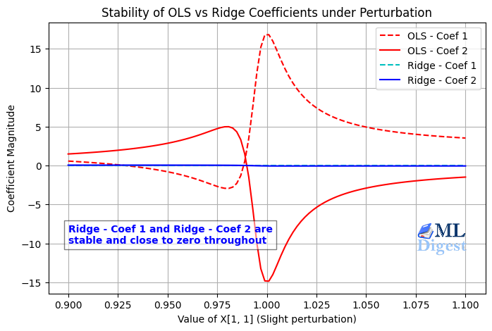
As can be seen, the OLS coefficients can be extremely large and unstable, while the ridge coefficients are much more balanced and stable. The predictions remain good in both cases, but ridge is more robust to the multicollinearity issue.

Bias-Variance Tradeoff

Ridge regression introduces bias, but it often reduces variance by much more than the amount of bias it adds.

That tradeoff is usually worth it when:

• Features are strongly correlated
• There are many features
• Coefficient stability matters
• Generalization matters more than perfectly unbiased estimates

The core idea is simple:

• OLS tries to fit the training data as closely as possible
• Ridge tries to fit the data while also discouraging large coefficients

This extra preference for smaller coefficients acts like a stabilizer.

Practical Guidance

In real projects, ridge regression works best when you follow a few implementation rules.

• Standardize Features First:
  Ridge penalizes coefficient magnitudes, so the scale of each feature matters. If one feature is measured in thousands and another in decimals, the penalty will affect them unevenly.
  That is why ridge is usually paired with feature standardization.
• Do Not Penalize the Intercept:
  Most libraries handle this correctly for you, but conceptually the intercept should not be shrunk in the same way as feature weights.
• Choose $\lambda$ with Cross-Validation:
  The regularization strength should usually be tuned on validation data rather than selected arbitrarily.
• Use Ridge When Prediction Stability Matters:
  If your goal is pure feature selection, lasso may be more appropriate. If your goal is stable estimation under correlated inputs, ridge is often a better fit.

When Ridge Helps Most

Ridge regression is especially useful when:

• You have many correlated numerical features
• You care about stable out-of-sample performance
• You want to keep all features instead of dropping some of them
• You suspect the instability is coming from variance rather than bias

It is common in linear models for tabular machine learning, polynomial regression, and high-dimensional settings where plain OLS becomes fragile.

Final Takeaway

Multicollinearity does not usually make OLS systematically wrong on average. It makes OLS unstable.

The instability comes from the fact that correlated features make $X^T X$ nearly singular. That makes $(X^T X)^{-1}$ large, which inflates the variance of coefficient estimates.

Ridge regression fixes this by replacing:

$$
X^T X \quad \text{with} \quad X^T X + \lambda I
$$

That simple change makes the matrix easier to invert, shrinks extreme coefficients, and produces a more stable model.