Imagine a teacher grading a multiple-choice exam. If the teacher says, “Only this one answer has any value, and all others are worth exactly zero,” the student may learn to become extremely confident, even when some alternatives are semantically similar. Label smoothing changes that teaching signal slightly. It still says which answer is correct, but it also leaves a tiny amount of probability mass for the other classes. That small change often leads to models that generalize better and behave less overconfidently.
In classification, one-hot labels tell the model that the true class has probability $1$ and every other class has probability $0$. Label smoothing softens that target just a little. The correct class still carries most of the probability mass, but the remaining classes receive a small share too.
At first glance, label smoothing looks almost too simple to matter. It modifies only the target distribution, not the architecture, not the optimizer, and not the forward pass. Yet that one modification changes the geometry of the learning problem and the gradients seen during training.
This article builds the idea in stages. It starts with intuition, then formalizes the method mathematically, derives the gradient with respect to the logits, and finally discusses when label smoothing helps, when it can hurt, and how to reason about it in practice.
1. What Label Smoothing Is
In ordinary multi-class classification, the target for each example is a one-hot vector. For a 4-class problem where class 2 is correct, the target is:
$$
\mathbf{y} = [0, 1, 0, 0]
$$
That vector says two things very aggressively:
- the correct class should receive probability $1$
- every incorrect class should receive probability $0$
Label smoothing replaces that hard target with a softened target:
$$
y_k^{\text{smooth}} = (1 – \epsilon) y_k + \frac{\epsilon}{K}
$$
where:
- $K$ is the number of classes
- $\epsilon$ is the smoothing strength
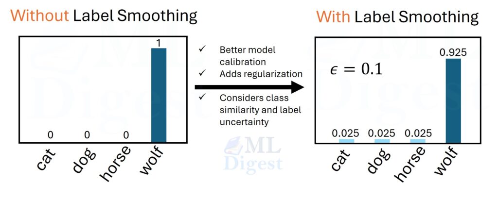
If $K = 4$ and $\epsilon = 0.1$, then the smoothed target becomes:
$$
\mathbf{y}^{\text{smooth}} = [0.025, 0.925, 0.025, 0.025]
$$
The correct class still dominates, but the target is no longer an extreme point of the simplex. That is the whole method.
1.1. A visual intuition
One-hot labels behave like a sharp spike: all probability mass sits on a single class. Label smoothing flattens that spike just a little. The model is still taught to prefer the correct class, but it is no longer rewarded for driving every alternative all the way to zero.
You can think of the picture this way: the one-hot target sits at a corner of the probability simplex, while the smoothed target is pulled slightly inward. Training is still directional, but it is no longer extreme.
1.2. Where label smoothing is commonly used
Label smoothing is most common in:
- image classification
- sequence classification
- language modeling with categorical targets
- speech recognition and speech classification
- large-scale transformer training
It is primarily a technique for single-label multi-class classification with softmax outputs.
2. Why This Small Change Matters
The easiest way to understand label smoothing is to ask what ordinary cross-entropy is trying to do. With one-hot targets, the model is trained to make the correct class probability approach $1$ and every other class probability approach $0$. In practice, that often means pushing logit gaps to become much larger than necessary.
Label smoothing weakens that pressure. The model must still identify the winner, but it is not encouraged to become infinitely certain.
2.1. It reduces overconfidence
Modern neural networks can be very accurate and still badly calibrated. A model may output $0.999$ confidence for examples that are not nearly that certain. One-hot training tends to amplify this behavior because the target itself is absolute.
Label smoothing changes the message from “assign all mass to the winner” to “assign most mass to the winner.” That tends to reduce the drive toward extreme probabilities.
2.2. It acts as target-side regularization
A helpful way to think about label smoothing is that it regularizes the training signal, not the parameters directly.
Weight decay says, “Do not let the parameters grow too freely.” Dropout says, “Do not rely too much on any one internal pathway.” Label smoothing says, “Do not fit the target as if it were infinitely certain.”
That often helps with:
- overfitting
- poor probability calibration
- noisy labels
- unnecessarily large logit margins
2.3. It better matches real datasets
Real datasets are rarely perfectly crisp.
- Some labels are wrong.
- Some classes overlap semantically.
- Some examples are genuinely ambiguous.
- Some annotation schemes force a single class even when the underlying signal is softer.
One-hot supervision assumes the opposite: complete certainty. Label smoothing injects a small amount of humility into the target distribution.
2.4. It changes the geometry of optimization
For a $K$-class classifier, the output distribution lies on a probability simplex. In a 3-class problem, that simplex is a triangle.
- one-hot targets lie at the corners
- smoothed targets lie slightly inside the triangle
That inward shift matters. The optimizer is no longer asked to hit the most extreme corners of the simplex. Instead, it is asked to match distributions in the interior. Geometrically, this means smaller required logit separations and less pressure to form excessively sharp decision surfaces.
3. The Mathematical Formulation
Let:
- $K$ be the number of classes
- $\mathbf{z} \in \mathbb{R}^K$ be the logits for one example
- $p_k$ be the softmax probability for class $k$
- $\mathbf{y}$ be the one-hot target
- $y^{\text{smooth}}$ be the smoothed target
The softmax probabilities are:
$$
p_k = \frac{e^{z_k}}{\sum_{j=1}^{K} e^{z_j}}
$$
The smoothed target is:
$$
y_k^{\text{smooth}} = (1 – \epsilon) y_k + \frac{\epsilon}{K}
$$
The cross-entropy loss for one example becomes:
$$
\mathcal{L} = -\sum_{k=1}^{K} y_k^{\text{smooth}} \log p_k
$$
3.1. What the target values become
Suppose class $c$ is the correct class.
For the correct class:
$$
y_c^{\text{smooth}} = 1 – \epsilon + \frac{\epsilon}{K}
$$
For any incorrect class $j \ne c$:
$$
y_j^{\text{smooth}} = \frac{\epsilon}{K}
$$
So label smoothing does two things simultaneously:
- it lowers the target assigned to the correct class
- it gives each incorrect class a small positive target
3.2. Alternative conventions
Some references use a slightly different definition:
$$
y_c^{\text{smooth}} = 1 – \epsilon, \qquad y_j^{\text{smooth}} = \frac{\epsilon}{K-1} \quad \text{for } j \ne c
$$
The intuition is the same. The total smoothing mass is still $\epsilon$, but it is distributed only among the incorrect classes.
This article uses the all-classes convention:
$$
y_k^{\text{smooth}} = (1 – \epsilon) y_k + \frac{\epsilon}{K}
$$
When comparing papers or libraries, always check which convention is being used. The numeric value of $\epsilon$ is not directly interchangeable across all definitions.
4. How Label Smoothing Changes Cross-Entropy
With ordinary one-hot labels, the loss for the correct class $c$ is:
$$
\mathcal{L}_{\text{one-hot}} = -\log p_c
$$
This objective rewards the model for pushing $p_c \to 1$, which usually means driving $z_c – z_j \to \infty$ for all $j \ne c$. The loss does not explicitly say “be calibrated.” It says “make the winner absolute.” That pressure can contribute to overconfident predictions, especially in over-parameterized models.
With label smoothing, the loss becomes:
$$
\mathcal{L}_{\text{smooth}} = -\sum_{k=1}^{K} y_k^{\text{smooth}} \log p_k
$$
Now the loss no longer depends only on the correct class probability. Every class participates, because every class has some target mass.
4.1. Information-theoretic interpretation
Let $U$ denote the uniform distribution over the $K$ classes, so that $U_k = 1/K$. Since
$$
\mathbf{y}^{\text{smooth}} = (1 – \epsilon) \mathbf{y} + \epsilon U,
$$
the smoothed loss can be written as:
$$
\mathcal{L}_{\text{smooth}} = (1 – \epsilon) \, CE(\mathbf{y}, \mathbf{p}) + \epsilon \, CE(U, \mathbf{p})
$$
and because
$$
CE(U, \mathbf{p}) = H(U) + KL(U || \mathbf{p}),
$$
where $H(U)$ is the entropy of the uniform distribution and $KL(U || \mathbf{p})$ is the KL divergence from $U$ to $\mathbf{p}$, we can further expand to get:
$$
\mathcal{L}_{\text{smooth}} = (1 – \epsilon) \, CE(\mathbf{y}, \mathbf{p}) + \epsilon \, KL(U || \mathbf{p}) + \epsilon \, H(U)
$$
The term $H(U)$ is constant with respect to the model, so for optimization purposes label smoothing is equivalent to combining:
$$
\mathcal{L}_{\text{smooth}} = (1 – \epsilon) \, CE(\mathbf{y}, \mathbf{p}) + \epsilon \, KL(U || \mathbf{p})
$$
- the usual hard-label cross-entropy, scaled by $(1-\epsilon)$
- a regularizer that discourages predictions from drifting too far away from the uniform distribution
This is the cleanest information-theoretic interpretation. Label smoothing does not simply replace cross-entropy with a heuristic softer loss. It adds a bias toward less concentrated output distributions.
What this means intuitively:
This decomposition explains why label smoothing often improves calibration. The model is still rewarded for assigning high probability to the correct class, but it is also softly penalized for making the distribution sharper than necessary.
This tends to reduce:
- extremely peaked output distributions
- oversized logit gaps
- brittle confidence estimates on the training set
It is not a guarantee of perfect calibration, but it often moves the model in the right direction.
4.2. Finite Optimal Logits
A crucial but often misunderstood mathematical property of label smoothing is that it bounds the optimal logit magnitudes. With one-hot targets, the minimum loss is achieved when $p_c \to 1$ and $p_j \to 0$, which requires the logit difference $z_c – z_j \to \infty$. The network is incentivized to make the logits infinitely large.
With label smoothing, the minimum loss is found exactly when the predicted probabilities match the softened targets: $p_k = y_k^{\text{smooth}}$.
Because the target probabilities are bounded away from $0$ and $1$, the optimal logit difference becomes finite:
$$
z_c^* – z_j^* = \log\left(\frac{p_c^*}{p_j^*}\right) = \log\left(\frac{1 – \epsilon + \epsilon/K}{\epsilon/K}\right)
$$
This mathematically proves why label smoothing reduces overconfidence—it structurally prevents the optimizer from blowing up the logit distances to infinity.
5. Deriving the Gradient with Respect to the Logits
This is the most important mathematical section because it shows exactly how the training signal changes.
We derive the gradient for a single example.
5.1. Setup
Let the logits be:
$$
\mathbf{z} = [z_1, z_2, \dots, z_K]
$$
and the softmax probabilities:
$$
p_k = \frac{e^{z_k}}{\sum_{m=1}^{K} e^{z_m}}
$$
The smoothed cross-entropy loss is:
$$
\mathcal{L} = -\sum_{k=1}^{K} y_k^{\text{smooth}} \log p_k
$$
We want:
$$
\frac{\partial \mathcal{L}}{\partial z_j}
$$
for any class $j$.
5.2. The key softmax identity
For softmax, a standard identity is:
$$
\frac{\partial \log p_k}{\partial z_j} = \delta_{kj} – p_j
$$
where $\delta_{kj}$ is the Kronecker delta:
$$
\delta_{kj} =
\begin{cases}
1 & \text{if } k = j \
0 & \text{if } k \ne j
\end{cases}
$$
5.3. Differentiate the loss
Start from:
$$
\mathcal{L} = -\sum_{k=1}^{K} y_k^{\text{smooth}} \log p_k
$$
Differentiate with respect to $z_j$:
$$
\frac{\partial \mathcal{L}}{\partial z_j} = -\sum_{k=1}^{K} y_k^{\text{smooth}} \frac{\partial \log p_k}{\partial z_j}
$$
Substitute the softmax identity:
$$
\frac{\partial \mathcal{L}}{\partial z_j}=-\sum_{k=1}^{K} y_k^{\text{smooth}} (\delta_{kj} – p_j)
$$
Distribute the sum:
$$
\frac{\partial \mathcal{L}}{\partial z_j}=-\sum_{k=1}^{K} y_k^{\text{smooth}} \delta_{kj} + \sum_{k=1}^{K} y_k^{\text{smooth}}
$$
Since $p_j$ does not depend on $k$, pull it out of the second sum:
$$
\frac{\partial \mathcal{L}}{\partial z_j}=-y_j^{\text{smooth}} + p_j \sum_{k=1}^{K} y_k^{\text{smooth}}
$$
Because the smoothed labels still form a probability distribution,
$$
\sum_{k=1}^{K} y_k^{\text{smooth}} = 1
$$
so the gradient simplifies to:
$$
\boxed{
\frac{\partial \mathcal{L}}{\partial z_j} = p_j – y_j^{\text{smooth}}
}
$$
Structurally, this is the same gradient form as ordinary cross-entropy. The only difference is that the target vector has changed.
5.4. Correct class versus incorrect classes
If $j = c$, then:
$$
\frac{\partial \mathcal{L}}{\partial z_c} = p_c – \left(1 – \epsilon + \frac{\epsilon}{K}\right)
$$
Without smoothing, the gradient would be:
$$
\frac{\partial \mathcal{L}}{\partial z_c} = p_c – 1
$$
So the correct-class gradient becomes less negative. Under gradient descent, that means the optimizer pushes the correct logit upward less aggressively.
If $j \ne c$, then:
$$
\frac{\partial \mathcal{L}}{\partial z_j} = p_j – \frac{\epsilon}{K}
$$
Without smoothing, the gradient would simply be:
$$
\frac{\partial \mathcal{L}}{\partial z_j} = p_j
$$
So each incorrect-class gradient is shifted downward by $\epsilon/K$.
This creates two regimes:
- If $p_j > \epsilon/K$, the gradient remains positive, so gradient descent pushes that incorrect logit downward.
- If $p_j < \epsilon/K$, the gradient becomes negative, so gradient descent nudges that incorrect logit upward slightly.
That second regime is the subtle but important one. Label smoothing does not train the model to annihilate all non-target probabilities. More precisely, it does not impose a hard floor on predicted probabilities at inference time; it changes the training target so that pushing every alternative all the way toward zero is no longer the preferred solution.
5.5. Side-by-side summary
For the correct class:
- one-hot: $p_c – 1$
- smoothed: $p_c – \left(1 – \epsilon + \epsilon/K\right)$
For an incorrect class:
- one-hot: $p_j$
- smoothed: $p_j – \epsilon/K$
One-hot training says, “make the winner absolute.” Label smoothing says, “make the winner clear, but not infinitely sharp.”
5.6. A Tiny Numerical Example
Suppose:
- $K = 5$
- the correct class is $c = 1$ (using 0-based indexing)
- $\epsilon = 0.1$
- the predicted probabilities are
$$
\mathbf{p} = [0.05, 0.80, 0.05, 0.06, 0.04]
$$
Then the smoothed target is:
$$
\mathbf{y}^{\text{smooth}} = [0.02, 0.92, 0.02, 0.02, 0.02]
$$
So the gradient is:
$$
\nabla_{\mathbf{z}} \mathcal{L} = \mathbf{p} – \mathbf{y}^{\text{smooth}} = [0.03, -0.12, 0.03, 0.04, 0.02]
$$
Without label smoothing, the one-hot target would be:
$$
\mathbf{y} = [0, 1, 0, 0, 0]
$$
and the gradient would be:
$$
\mathbf{p} – \mathbf{y} = [0.05, -0.20, 0.05, 0.06, 0.04]
$$
The difference is easy to read:
- the correct logit receives a weaker upward push
- the incorrect logits receive weaker downward pushes
- the entire update is softer and less extreme
That is the optimization effect of label smoothing in one line.
6. Why It Often Improves Generalization and Calibration
Label smoothing does not magically make a model smarter. What it often does is prevent the model from learning an unnecessarily brittle version of the task.
6.1. Better calibrated probabilities
Many modern classifiers are accurate but poorly calibrated. They may predict 0.999 even when they should be less certain.
Label smoothing often improves calibration because it trains the model against a less extreme target distribution.
6.2. Less brittle internal representations
When a model is pushed toward absolute certainty on the training set, it may learn features that are sharper than necessary. Those representations can be sensitive to nuisance variation and small perturbations.
Label smoothing can encourage more compact class clusters and more moderate margins in representation space.
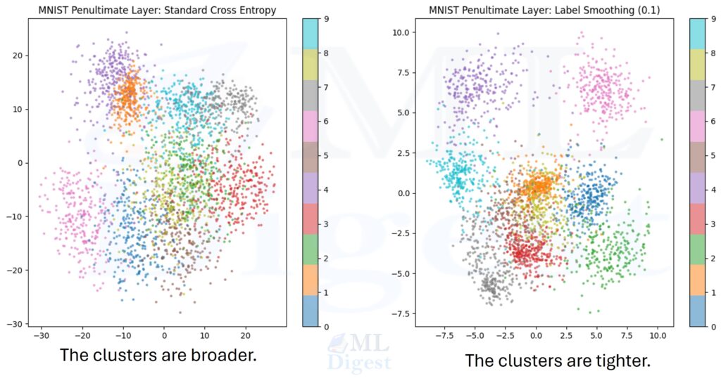
The above image shows the clustering of penultimate layer representations in a 2D projection (check this paper for details). The main intuition is that one-hot training can produce broader or less organized class regions, while label smoothing can encourage tighter within-class clustering and clearer separation across categories. That is one plausible route to better generalization.
6.3. Reduced pressure to memorize noisy labels
If a portion of the training set is mislabeled, one-hot cross-entropy can fit those examples very aggressively. Label smoothing lowers that pressure because even the target distribution itself admits some uncertainty.
This is not a full solution to label noise, but it can be a useful buffer.
6.4. An important caveat
Label smoothing often improves calibration, but not always. In some settings it can make the model under-confident, especially when combined with other strong regularizers or heavy target-softening techniques such as mixup. The correct mental model is not “label smoothing is always better,” but “label smoothing shifts the confidence profile, often in a helpful direction.”
7. When to Use It and When to Avoid It
Label smoothing is usually a good candidate when:
- the task is single-label multi-class classification
- the model is visibly overconfident
- the dataset is large enough that regularization is helpful
- probability calibration matters alongside accuracy
- the labels are somewhat noisy or ambiguously defined
Be careful or skip it when:
- the task is multi-label classification with independent sigmoids
- the target distribution is already soft and meaningful
- the task requires preserving very sharp probabilities
- the model is already under-confident
- several other techniques are already softening the targets or outputs
- a large $\epsilon$ would blur distinctions that the task genuinely needs
The guiding question is simple: is the target distribution supposed to encode certainty, or only a supervised preference? Label smoothing helps more in the second case than in the first.
8. How to Choose the Smoothing Value
The most common starting values are:
- $\epsilon = 0.05$
- $\epsilon = 0.1$
Sometimes larger values such as $0.2$ appear in very large-scale or noisy settings, but they are not safe defaults.
The trade-off is straightforward:
- too small, and the effect may be negligible
- too large, and the model may become under-confident or lose accuracy
In practice, $0.1$ is a strong default for a first experiment, but it should still be validated rather than assumed.
One useful diagnostic is to monitor both accuracy and calibration. If top-1 accuracy changes little while negative log-likelihood or expected calibration error improves, the smoothing strength may be doing exactly what it should.
9. Implementation
In modern libraries, the built-in implementation is usually the best choice because it is stable, simple, and easy to audit.
9.1. Built-in loss
import torch
import torch.nn as nn

batch_size = 8
num_classes = 5

logits = torch.randn(batch_size, num_classes, requires_grad=True)
targets = torch.randint(0, num_classes, size=(batch_size,))

criterion = nn.CrossEntropyLoss(label_smoothing=0.1)
loss = criterion(logits, targets)
loss.backward()

print("loss:", float(loss))
print("gradient shape:", logits.grad.shape)
# The exact loss value will differ from run to run unless you set a random seed.
# The gradient shape will be: torch.Size([8, 5])Two practical reminders:
- pass raw logits, not softmax probabilities
- evaluate accuracy against the original hard labels
9.2. Implementing label smoothing from scratch
Writing the loss manually is useful for learning, debugging, or custom research code.
import torch
import torch.nn.functional as F

def cross_entropy_with_label_smoothing(logits, targets, epsilon=0.1):
    """
    logits:  [batch_size, num_classes]
    targets: [batch_size] with integer class ids
    """
    num_classes = logits.size(1)
    log_probs = F.log_softmax(logits, dim=1)

    with torch.no_grad():
        true_dist = torch.full_like(log_probs, epsilon / num_classes)
        true_dist.scatter_(
            1,
            targets.unsqueeze(1),
            1.0 - epsilon + epsilon / num_classes,
        )

    loss = -(true_dist * log_probs).sum(dim=1).mean()
    return loss


batch_size = 4
num_classes = 3

logits = torch.tensor(
    [
        [2.0, 0.5, -1.0],
        [0.1, 1.8, 0.2],
        [1.2, 0.7, 0.3],
        [0.0, -0.2, 2.4],
    ],
    requires_grad=True,
)

targets = torch.tensor([0, 1, 0, 2])

loss = cross_entropy_with_label_smoothing(logits, targets, epsilon=0.1)
loss.backward()

print("loss:", float(loss))
print("gradients:\n", logits.grad)
# Expected output:
#     loss: 0.47310787439346313
#     gradients:
#     tensor([[-0.0369,  0.0355,  0.0014],
#             [ 0.0247, -0.0528,  0.0281],
#             [-0.1091,  0.0670,  0.0422],
# [ 0.0111, 0.0076, -0.0187]])The manual implementation is especially helpful because you can inspect true_dist directly and verify that the targets are being constructed exactly as intended.
10. Practical Workflow and Common Mistakes
The easiest way to use label smoothing well is to treat it like any other regularizer: change one thing, keep the comparison clean, and measure what actually improved.
10.1. A simple workflow
- Train a baseline with ordinary cross-entropy.
- Add label smoothing with $\epsilon = 0.05$ or $0.1$.
- Keep the optimizer, learning-rate schedule, augmentation, and architecture fixed.
- Compare validation accuracy, negative log-likelihood, and calibration.
- Tune $\epsilon$ only if the initial comparison justifies it.
10.2. What to monitor
Beyond top-1 accuracy, inspect:
- validation loss
- negative log-likelihood
- expected calibration error
- reliability diagrams
- confidence histograms
If accuracy stays similar while calibration improves, label smoothing may still be a net win.
10.3. Common mistakes
- using too large an $\epsilon$
- applying it to the wrong task type
- passing probabilities instead of logits into cross-entropy
- comparing smoothed and unsmoothed training losses without context
- forgetting that different papers and libraries use different smoothing conventions
- applying smoothing on top of already soft targets without a clear reason
10.4. Interactions with other techniques
Label smoothing often works well with:
- weight decay
- dropout
- data augmentation
It can also be combined with mixup or cutmix, but that combination needs extra care because those methods already soften the supervision signal.
But regularizers accumulate. If several components already soften the training signal, extra smoothing can become redundant or make the model too cautious.
10.5. Sequence models need an extra check
In NLP or speech pipelines, some positions correspond to padding or ignored tokens. Smoothing should be applied only to valid targets, and ignored positions should remain excluded from the loss. Otherwise the training signal becomes subtly wrong.
11. Relationship to Nearby Ideas
Label smoothing is close to several other techniques, but it is not interchangeable with them.
11.1. Confidence penalty
Instead of smoothing labels, a confidence penalty adds an entropy-based regularizer to the loss:
$$
\mathcal{L} = CE – \lambda H(\mathbf{p})
$$
where $H(\mathbf{p})$ is the entropy of the predicted distribution.
Conceptually:
- label smoothing changes the target distribution
- confidence penalty changes the objective directly by discouraging low-entropy predictions
Both aim to reduce excessive certainty, but they do so from different angles.
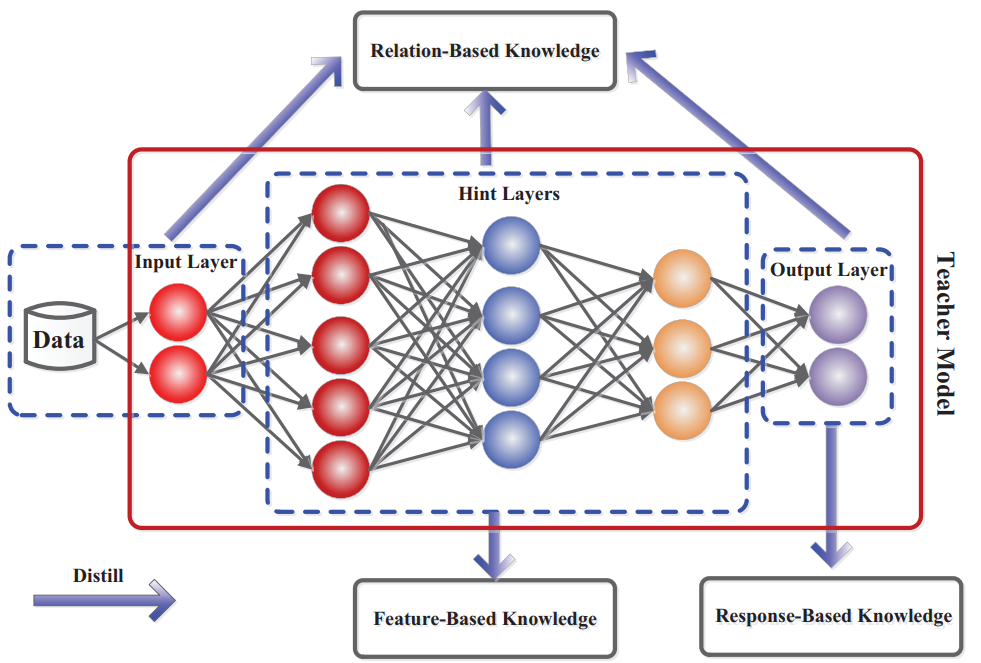
11.2. Knowledge distillation
Distillation uses a teacher model to provide example-specific soft targets.
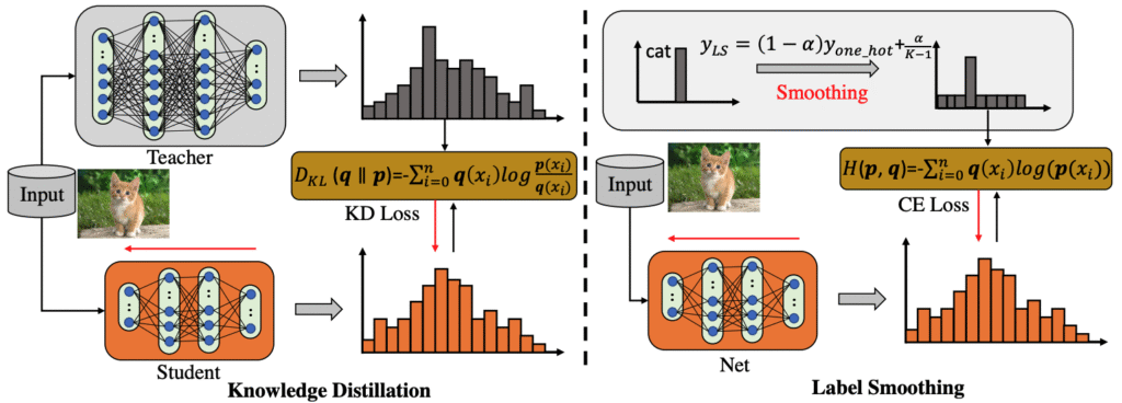
Label smoothing, by contrast, usually uses a fixed prior-like target adjustment, often uniform across classes. It does not encode the teacher’s example-specific beliefs about which alternatives are plausible.
11.3. Mixup
Mixup creates soft labels by interpolating two training examples and their labels. In that case, the softness comes from the data construction itself.
Label smoothing changes only the targets. The input remains unchanged.
11.4. Why not just use label smoothing for a teacher during knowledge distillation?
A teacher trained with label smoothing can achieve better standalone accuracy and still transfer less useful information to a student than a teacher trained on hard targets.
The intuition is mathematically profound. Label smoothing encourages the teacher to preserve the main class distinction, but forces the predicted probabilities of all incorrect classes to converge toward the exact same value ($\epsilon/K$). This effectively artificially flattens the distribution and destroys the variance between incorrect classes.
In standard one-hot training, a network might assign slightly higher probability to “dog” than “airplane” when shown a “cat”, because dogs are visually and semantically closer. This is often called “dark knowledge.” Label smoothing penalizes this natural similarity, aggressively pulling both “dog” and “airplane” predictions to $\epsilon/K$. Because it actively erases these fine-grained relative similarities, a teacher trained with label smoothing becomes a less informative instructor for distillation, even if its own generalization improves.
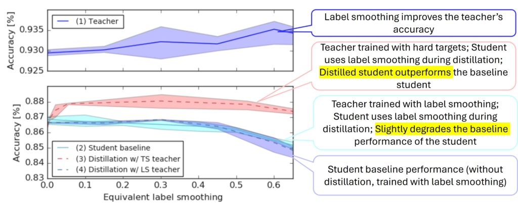
As shown in the above figure from this paper, a teacher trained with hard targets can transfer more knowledge to a student than a teacher trained with label smoothing, even if the smoothed teacher has better standalone accuracy. The student learns more from the richer, less smoothed output distribution of the hard-target teacher, where the natural “dark knowledge” remains intact.
12. Variants of Label Smoothing
Standard uniform label smoothing is the most common version, but it is not the only one.
Class-dependent smoothing:
Not every wrong class is equally plausible. In some domains, domain knowledge or a confusion matrix can justify assigning more mass to classes that are semantically close to the target.
For example, “cat” may reasonably share more smoothing mass with “dog” than with “airplane.”
Adaptive smoothing:
Instead of using a fixed $\epsilon$, adaptive methods vary the smoothing strength based on the training step, example difficulty, or model confidence.
These methods can be more flexible, but they are also harder to tune and explain.
Soft targets from other sources:
If the target distribution already comes from a teacher model, weak supervision, or annotation aggregation, standard label smoothing may not be appropriate. In that case, you already have a soft target, and additional smoothing can distort useful information.
13. Summary
Label smoothing is a small change with a large conceptual payoff. It replaces a one-hot target with a slightly softened target, so the model is asked to be correct without becoming maximally certain.
The core equation is:
$$
y_k^{\text{smooth}} = (1 – \epsilon) y_k + \frac{\epsilon}{K}
$$
and the key gradient result is:
$$
\boxed{\frac{\partial \mathcal{L}}{\partial z_j} = p_j – y_j^{\text{smooth}}}
$$
That single gradient formula explains the main behavior:
- the correct class is pushed upward less aggressively
- the incorrect classes are pushed downward less aggressively
- the optimizer is discouraged from creating unnecessarily sharp distributions
That is why label smoothing often improves calibration and can improve generalization.
If you remember only one sentence, remember this one: label smoothing tells a classifier, “Be confident enough to decide, but not so confident that it stops respecting uncertainty.”

Happy is a seasoned ML professional with over 15 years of experience. His expertise spans various domains, including Computer Vision, Natural Language Processing (NLP), and Time Series analysis. He holds a PhD in Machine Learning from IIT Kharagpur and has furthered his research with postdoctoral experience at INRIA-Sophia Antipolis, France. Happy has a proven track record of delivering impactful ML solutions to clients.
Subscribe to our newsletter!