Mixture of Experts (MoE): Scaling Model Capacity Without Proportional Compute

Imagine you are building a house.

You could hire one master builder who knows everything about construction, from plumbing and electrical wiring to masonry and carpentry. This builder would be knowledgeable, but expensive, and they would lose time switching between very different tasks.

Now imagine hiring a general contractor instead. The contractor coordinates specialists: a plumber, an electrician, a carpenter, and a mason. When plumbing work arrives, the plumber takes it. When wiring work arrives, the electrician takes it. You still have access to a large pool of skills, but you pay for (and execute) only the specialties needed for each task.

That is the core intuition behind Mixture of Experts (MoE) models.

An MoE layer contains many expert subnetworks (usually feed-forward networks), plus a router (also called a gating network) that decides, for each token, which small subset of experts should process it. The key promise is more total capacity (more parameters stored across all experts) while keeping per-token compute roughly similar to a much smaller dense model.

This article builds intuition first, then moves into the mechanics: routing, capacity limits, load balancing, and the systems constraints that make (or break) MoE in practice.

Why Mixture of Experts? Capacity Without Proportional Compute

In the world of deep learning, there has been a consistent trend: bigger models, trained on more data, tend to perform better. The Transformer architecture, which powers models like GPT, is a perfect example. As we increase the number of parameters in a Transformer, its ability to understand and generate nuanced language improves.

However, this scaling comes at a steep price. A standard dense Transformer uses (almost) all of its parameters for every token. If you double the number of parameters in the feed-forward blocks, you roughly double the amount of computation (and thus time and cost) required for those blocks at training and inference. This makes scaling to trillions of parameters economically and computationally infeasible for dense models.

MoE offers a way out of this trap. It decouples parameter count from compute cost. It allows us to increase a model’s capacity (total parameters) significantly without proportionally increasing the computation per token. It does this via sparse activation: only a small subset of experts is active for each token.

The Core Idea: Replace One Big FFN With Many Small FFNs

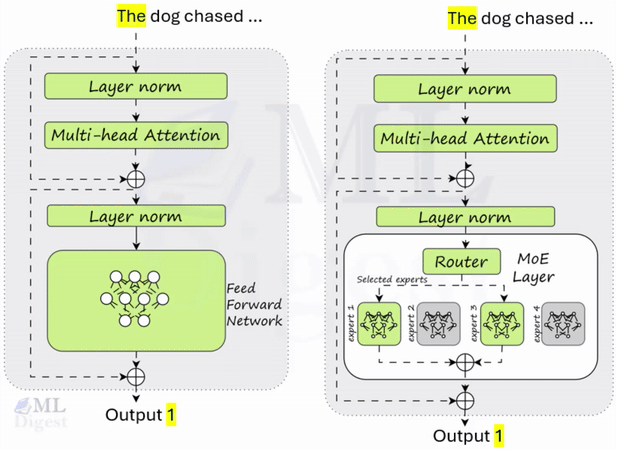
Let us visualize how an MoE layer sits inside a Transformer. In a standard Transformer, the feed-forward network (FFN) block is dense. Every token uses the same FFN parameters.

An MoE layer replaces that dense FFN with a collection of smaller FFNs (the experts) plus a small router (the gating network).

When a token arrives at the MoE layer:

1. The gating network examines the token and decides which of the experts are best suited to process it. It assigns a “score” or probability to each expert.
2. Based on these scores, only the Top-$k$ experts (typically $k=2$) are selected to process the token. All other experts remain inactive.
3. The token is processed by the selected experts.
4. The outputs of the active experts are combined, usually through a weighted sum based on the scores from the gating network.

This is the magic of sparse activation: you can store a very large number of parameters across experts, but each token only computes a small slice of them.

There are two costs worth separating:

• Compute (FLOPs): scales with the number of active experts per token (for example, $k=1$ or $k=2$).
• Memory and bandwidth: you still need the expert weights available somewhere (GPU memory, CPU memory, or across devices). Systems engineering decides whether those weights are replicated, sharded, paged, or routed across workers.

Thus, even if an MoE layer has, for example, 128 experts and a total of 180 billion parameters, each token only activates a tiny fraction of them (for example, $k=2$ experts with a combined 2.8 billion parameters). The model has a massive capacity to store knowledge, but it attempts to keep per-token compute bounded.

Diving Deeper: The Architecture of an MoE Layer

An MoE layer has two moving parts: experts and a router.

1) The Experts

The “experts” themselves are typically simple neural networks. In the context of a Transformer, each expert is usually a standard feed-forward network (FFN), consisting of multiple linear layers with a non-linear activation function in between (like ReLU or GeLU).

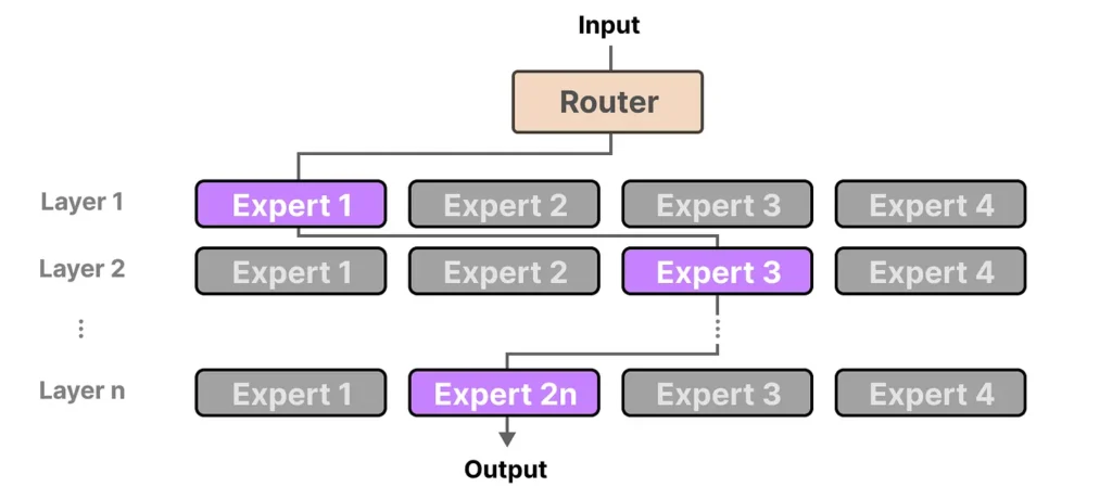
All experts usually share the same architecture but have different weights. During training, specialization often emerges: some experts get activated more for code-like tokens, others for multilingual text, others for certain stylistic patterns. This is not guaranteed, but it is a common empirical observation when the router is well-regularized and capacity is sufficient.

2) The Router (Gating Network)

The gating network is the brain of the operation. Its job is to look at an input token and decide which expert(s) should handle it. It is a small neural network, often just a single linear layer, that takes the token’s embedding as input.

For an input token embedding \(x \in \mathbb{R}^{d}\), the router outputs logits over experts. Intuitively, each logit measures how suitable an expert is for processing that token.

$$\text{logits} = \text{Router}(x)$$

To turn these logits into a probabilistic distribution (i.e., scores that sum to 1), a softmax function is applied.

$$\text{scores} = \text{softmax}(\text{logits})$$
The router is trained jointly with the rest of the model. In practice, the router is also where many MoE-specific tricks live: top-$k$ selection, capacity limits per expert, auxiliary load-balancing losses, and sometimes router noise.

3) Capacity, Dropped Tokens, and Why It Matters

In real MoE training and inference, each expert typically has a capacity: the maximum number of tokens it is allowed to process for a given forward pass. Capacity exists to make memory use predictable and to prevent a single overloaded expert from becoming a step-time straggler.

Capacity is commonly set proportional to the expected number of routed tokens per expert:

$$\text{capacity} = \left\lceil \text{capacity_factor} \cdot \frac{T \cdot k}{n} \right\rceil$$

where $T$ is the number of tokens in the (micro)batch, $k$ is the number of experts per token, and $n$ is the number of experts.

If more than capacity tokens route to an expert, implementations must choose a policy:

• Drop tokens: overflow tokens do not get that expert computation (quality can degrade).
• Reroute tokens: overflow goes to the next-best expert (more compute and more routing overhead).
• Increase capacity: fewer drops, but higher memory use and and slows down the model; potentially worse imbalance.

This capacity constraint is a major reason that load balancing is operationally important, not merely aesthetic.

The Mathematics Behind Mixture of Experts

Let there be $n$ experts, $E_1, \ldots, E_n$. For a token embedding $x$:

1. Router scores: the router produces a distribution over experts. $$ g = \text{softmax}(W_g x) \in \mathbb{R}^{n} $$ Here, $W_g$ is the weight matrix of the linear layer in the gating network.
2. Expert outputs: expert $i$ produces $o_i = E_i(x)$.
3. Mixture output: The final output ($y$) of the MoE layer is a weighted sum of the individual expert outputs: $$ y = \sum_{i=1}^{n} g_i\, o_i = \sum_{i=1}^{n} g_i\, E_i(x)$$

This formula describes a “soft” MoE where every expert contributes to the output, weighted by its score. It is conceptually clean but computationally expensive because it evaluates all $n$ experts.

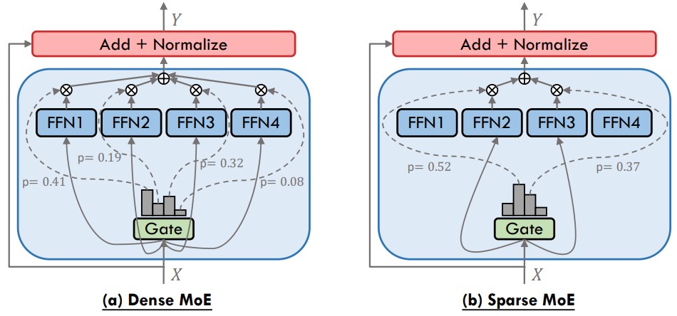
(An MoE layer in Transformers routes each input through a gating network that selects either all experts (Dense MoE) or only the top-k experts (Sparse MoE), and combines their outputs weighted by the gate’s softmax scores.[Image source])

Sparsity: Top-$k$ Routing

To get an MoE that is both large and fast, we pick only the top-$k$ experts per token (often $k=1$ or $k=2$).

The sparse mixture can be written as:

1. Compute router probabilities $g = \text{softmax}(W_g x)$.
2. Choose the set of indices $I$ corresponding to the top-$k$ values in $g$.
3. Keep only probabilities for $i \in I$ and (optionally) renormalize them so they sum to 1.

Then the output is:

$$ y = \sum_{i \in I} \tilde{g}_i\,E_i(x) $$

where $\tilde{g}$ is the masked (and possibly renormalized) gate value.

A Note on Differentiability:
You might wonder: “Is the Top-k operation differentiable?” The selection of indices itself is discrete and non-differentiable. However, the values of the gate $\tilde{g}_i$ and the expert outputs $E_i(x)$ are differentiable. During backpropagation, gradients flow through the weighted sum to the selected experts and the router weights that produced the scores for those experts. Experts that are not selected receive no gradient for that token. This is why auxiliary losses are vital—they ensure the router learns to use all experts, preventing some from “starving” without gradients.

The Load Balancing Loss (Preventing Expert Collapse)

A critical challenge is expert collapse: the router can develop a favorite expert and send a disproportionate number of tokens to it. The result is worse quality and wasted parameters, because unused experts do not learn.

To mitigate this, many MoE systems add a load-balancing auxiliary loss that encourages the router to spread traffic. The goal is not perfect uniformity for its own sake; the goal is to prevent a few experts from becoming bottlenecks while other experts never learn.

One popular form (used in Switch Transformers and related work) uses two batch-level statistics:

• $f_i$: fraction of tokens actually routed to expert $i$ (after top-$k$ selection and any capacity constraints)
• $p_i$: average router probability mass assigned to expert $i$

Then the auxiliary objective is

$$ \mathcal{L}_{\text{lb}} = \alpha\, n \sum_{i=1}^{n} f_i\,p_i $$
where $\alpha$ is a scaling hyperparameter.
This loss is minimized (approximately) when each expert receives an equal number of tokens and is assigned a similar amount of probability mass. This ensures that all experts are utilized and continue to learn during training.

Note: individual implementations differ. Some add router noise (to encourage exploration early), a z-loss term on router logits (to control logit scale), or different definitions of $f$ depending on whether tokens are counted before or after capacity constraints are applied.

Expert Choice Routing (Flip the Decision: Experts Pick Tokens)

Token-choice routing answers the question: for each token, which expert should process it? This feels natural, but it has an awkward failure mode: many tokens can pile onto the same expert, which forces capacity tricks (dropping, rerouting) and creates stragglers.

Expert choice routing flips the direction of the assignment.

Instead of tokens competing for experts, experts compete for tokens.

Here is the intuition to keep in mind:

• In token-choice, the router produces a Top-$k$ experts list per token.
• In expert-choice, the router produces a Top-$k$ tokens list per expert.

That simple flip makes capacity control feel built-in: each expert takes at most $m$ tokens, by design.

There are two common combination conventions:

• Fan-in (tokens may be chosen by multiple experts): if a token is selected by multiple experts, sum (or average) their contributions with weights derived from the router scores.
• Enforce exactly-$k$ experts per token: add a constraint or post-processing so each token is processed by exactly $k$ experts.

Why This Can Be Easier to Balance

In token-choice routing, capacity is an afterthought: tokens choose experts, then you impose per-expert capacity and handle overflow. In expert-choice routing, capacity is the selection rule itself: each expert selects exactly $k$ tokens.

This tends to reduce:

• Expert overload and token dropping: fewer “too many tokens for one expert” situations.
• Step-time stragglers: more uniform token counts per expert can reduce tail latency in training.

However, expert choice routing introduces its own trade-offs:

• Token coverage: some tokens might not be selected by any expert unless you enforce coverage.
• Extra coordination: if you want exactly $k$ experts per token, you need a mechanism that resolves collisions and guarantees coverage.

Other MoE Optimization Methods

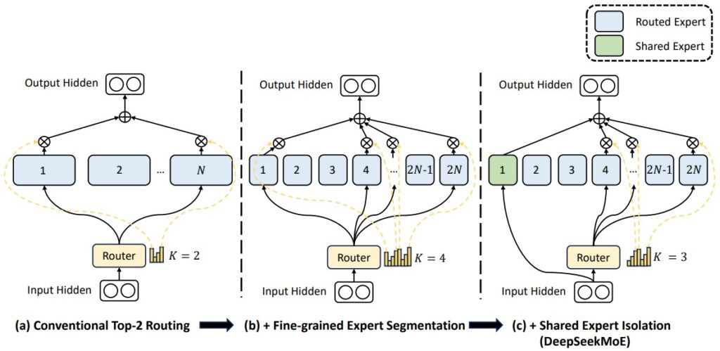
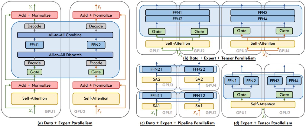
Many systems optimizations exist to improve MoE performance, which are beyond this article’s scope. A few highlights can be found in this work.

Routing as a Systems Problem (What the Equations Do Not Show)

The core computation $y = \sum_{i \in I} \tilde{g}_i E_i(x)$ is clean. The path to compute it efficiently at scale is often dominated by dispatch and communication.

When experts are sharded across devices (expert parallelism), a typical forward pass looks like this:

1. Score and select: compute router logits and Top-$k$ indices for each token.
2. Dispatch: group tokens by selected expert.
3. All-to-all: send token groups to the devices that host the target experts.
4. Expert compute: each device runs its local experts on the incoming token batches.
5. Combine: return outputs, apply gate weights, and restore original token order.

This is why MoE can be throughput-efficient while still feeling latency-sensitive: the fixed overheads (routing, reshaping, all-to-all) can dominate when batch sizes are small.

Implementing an MoE Layer

The following code provides a simplified, educational implementation of an MoE layer in PyTorch. It demonstrates the core mechanics: the router, the expert selection, and the weighted combination of outputs.

Note: Real-world MoE implementations (like those in Megatron-LM or DeepSpeed) are highly optimized for GPU performance. They avoid explicit Python loops over tokens and use specialized kernels (like scatter and gather operations) to efficiently route tokens to experts in parallel.

import torch
import torch.nn as nn
import torch.nn.functional as F

class Expert(nn.Module):
    """A simple feed-forward network expert."""
    def __init__(self, d_model, d_hidden):
        super().__init__()
        self.net = nn.Sequential(
            nn.Linear(d_model, d_hidden),
            nn.ReLU(),
            nn.Linear(d_hidden, d_model)
        )

    def forward(self, x):
        return self.net(x)

class MoELayer(nn.Module):
    """A Mixture of Experts layer with Top-k routing."""
    def __init__(self, d_model, num_experts, top_k, d_hidden):
        super().__init__()
        self.d_model = d_model
        self.num_experts = num_experts
        self.top_k = top_k

        # Create the expert networks
        self.experts = nn.ModuleList([Expert(d_model, d_hidden) for _ in range(num_experts)])

        # Router (gating network)
        self.router = nn.Linear(d_model, num_experts)

    def forward(self, x):
        # x has shape: (batch_size, seq_len, d_model)
        batch_size, seq_len, d_model = x.shape

        # Reshape for routing: (batch_size * seq_len, d_model)
        x_flat = x.view(-1, d_model)

        # Router logits: (batch_size * seq_len, num_experts)
        router_logits = self.router(x_flat)

        # Router probabilities per token
        router_probs = F.softmax(router_logits, dim=-1)

        # Select top-k experts for each token
        top_k_weights, top_k_indices = torch.topk(router_probs, k=self.top_k, dim=-1)

        # Renormalize weights over the selected experts
        top_k_weights = top_k_weights / (top_k_weights.sum(dim=-1, keepdim=True) + 1e-9)

        # Initialize final output tensor
        final_output = torch.zeros_like(x_flat)

        # Educational (slow) routing loop.
        # Each token is processed by top-k experts and weighted-summed.
        for token_idx in range(x_flat.size(0)):
            token = x_flat[token_idx].unsqueeze(0)
            for j in range(self.top_k):
                expert_idx = int(top_k_indices[token_idx, j].item())
                weight = top_k_weights[token_idx, j]
                expert_out = self.experts[expert_idx](token).squeeze(0)
                final_output[token_idx] += weight * expert_out

        # Reshape back to original shape: (batch_size, seq_len, d_model)
        return final_output.view(batch_size, seq_len, d_model)

# Example Usage
d_model = 512
num_experts = 8
top_k = 2
d_hidden = 2048
batch_size = 4
seq_len = 10

moe_layer = MoELayer(d_model, num_experts, top_k, d_hidden)
input_tensor = torch.randn(batch_size, seq_len, d_model)
output = moe_layer(input_tensor)

print("Input shape:", input_tensor.shape) # Input shape: torch.Size([4, 10, 512])
print("Output shape:", output.shape) # Output shape: torch.Size([4, 10, 512])


def count_parameters(model):
    return sum(p.numel() for p in model.parameters() if p.requires_grad)

# Total parameters
total_params = count_parameters(moe_layer)
print(f"Total number of parameters in MoELayer: {total_params:,}") # Total number of parameters in MoELayer: 16,801,800

# Active parameters during inference (per token)
# This includes the gating network always, plus the top_k experts.

# Router parameters
router_params = sum(p.numel() for p in moe_layer.router.parameters() if p.requires_grad)

# Parameters for a single expert
# Assuming all experts have the same structure
params_per_expert = count_parameters(moe_layer.experts[0])

# Active parameters = Gating network params + (top_k * params_per_expert)
active_params_per_token = router_params + (top_k * params_per_expert)

print(f"Active parameters during inference (per token): {active_params_per_token:,}")

import torch
import torch.nn as nn
import torch.nn.functional as F

class Expert(nn.Module):
    """A simple feed-forward network expert."""
    def __init__(self, d_model, d_hidden):
        super().__init__()
        self.net = nn.Sequential(
            nn.Linear(d_model, d_hidden),
            nn.ReLU(),
            nn.Linear(d_hidden, d_model)
        )

    def forward(self, x):
        return self.net(x)

class MoELayer(nn.Module):
    """A Mixture of Experts layer with Top-k routing."""
    def __init__(self, d_model, num_experts, top_k, d_hidden):
        super().__init__()
        self.d_model = d_model
        self.num_experts = num_experts
        self.top_k = top_k

        # Create the expert networks
        self.experts = nn.ModuleList([Expert(d_model, d_hidden) for _ in range(num_experts)])

        # Router (gating network)
        self.router = nn.Linear(d_model, num_experts)

    def forward(self, x):
        # x has shape: (batch_size, seq_len, d_model)
        batch_size, seq_len, d_model = x.shape

        # Reshape for routing: (batch_size * seq_len, d_model)
        x_flat = x.view(-1, d_model)

        # Router logits: (batch_size * seq_len, num_experts)
        router_logits = self.router(x_flat)

        # Router probabilities per token
        router_probs = F.softmax(router_logits, dim=-1)

        # Select top-k experts for each token
        top_k_weights, top_k_indices = torch.topk(router_probs, k=self.top_k, dim=-1)

        # Renormalize weights over the selected experts
        top_k_weights = top_k_weights / (top_k_weights.sum(dim=-1, keepdim=True) + 1e-9)

        # Initialize final output tensor
        final_output = torch.zeros_like(x_flat)

        # Educational (slow) routing loop.
        # Each token is processed by top-k experts and weighted-summed.
        for token_idx in range(x_flat.size(0)):
            token = x_flat[token_idx].unsqueeze(0)
            for j in range(self.top_k):
                expert_idx = int(top_k_indices[token_idx, j].item())
                weight = top_k_weights[token_idx, j]
                expert_out = self.experts[expert_idx](token).squeeze(0)
                final_output[token_idx] += weight * expert_out

        # Reshape back to original shape: (batch_size, seq_len, d_model)
        return final_output.view(batch_size, seq_len, d_model)

# Example Usage
d_model = 512
num_experts = 8
top_k = 2
d_hidden = 2048
batch_size = 4
seq_len = 10

moe_layer = MoELayer(d_model, num_experts, top_k, d_hidden)
input_tensor = torch.randn(batch_size, seq_len, d_model)
output = moe_layer(input_tensor)

print("Input shape:", input_tensor.shape) # Input shape: torch.Size([4, 10, 512])
print("Output shape:", output.shape) # Output shape: torch.Size([4, 10, 512])


def count_parameters(model):
    return sum(p.numel() for p in model.parameters() if p.requires_grad)

# Total parameters
total_params = count_parameters(moe_layer)
print(f"Total number of parameters in MoELayer: {total_params:,}") # Total number of parameters in MoELayer: 16,801,800

# Active parameters during inference (per token)
# This includes the gating network always, plus the top_k experts.

# Router parameters
router_params = sum(p.numel() for p in moe_layer.router.parameters() if p.requires_grad)

# Parameters for a single expert
# Assuming all experts have the same structure
params_per_expert = count_parameters(moe_layer.experts[0])

# Active parameters = Gating network params + (top_k * params_per_expert)
active_params_per_token = router_params + (top_k * params_per_expert)

print(f"Active parameters during inference (per token): {active_params_per_token:,}")

MoE in the Wild: Famous Architectures

The Mixture of Experts concept has been the driving force behind some of the largest and most powerful language models to date.

1. Google’s GLaM (Generalist Language Model): One of the first modern models to showcase the power of MoE at scale, GLaM (2021) was a 1.2 trillion parameter model. However, it only activated about 97 billion parameters per token, making it computationally comparable to the much smaller GPT-3 (175B).
2. Switch Transformers: Also from Google, the Switch Transformer (2021) pushed the MoE concept further by simplifying the routing to k=1. Each token is sent to only one expert. This is computationally very efficient but requires careful load balancing. They trained models up to 1.6 trillion parameters.
3. Mistral’s Mixtral 8x7B: A highly popular and powerful open-source model, Mixtral 8x7B (2023) uses 8 experts and selects 2 per token. Its total parameter (47 billion) count is much larger than its per-token active parameters (13 billion), which helps it achieve strong quality at relatively low inference cost.
4. Databricks DBRX: DBRX (2024) is another powerful open-source MoE model. It has 132B total parameters but only activates 36B per token. It uses a more fine-grained MoE architecture with 16 experts, of which 4 are selected for each token.

When MoE Helps (And When It Hurts)

MoE is best understood as a trade: you exchange dense compute for sparse compute plus routing and communication.

Where MoE tends to shine

• Compute-limited regimes: if you are FLOP-limited, adding experts can buy quality while keeping $k$ small.
• Diverse training mixtures: specialization pressure is stronger when the data spans domains (code, math, multilingual, instruction tuning).

Where MoE can disappoint

• Latency-sensitive inference at small batch sizes: routing and communication overheads can dominate.
• Bandwidth-limited clusters: expert parallelism relies on fast interconnect; slow all-to-all erases gains.
• Unstable routing: without balancing and capacity management, a few experts do most of the work and quality suffers.

Practical Tips and Considerations

• Expert specialization is not guaranteed: specialization can emerge, but it depends on router regularization, data diversity, and sufficient capacity. Routing histograms often reveal whether experts are meaningfully distinct or merely load-balanced copies.
• Track token drops and overflow: capacity constraints can drop overflow tokens or force rerouting. Track drop rates explicitly; even small sustained drop rates can show up as evaluation regressions.
• Fine-tuning can destabilize routing: fine-tuning shifts token distributions. If the router learns too quickly, it can collapse to a subset of experts and sometimes it is beneficial to freeze the gating network while fine-tuning the experts on a specific task. A common mitigation is a smaller learning rate for the router or freezing it early, then unfreezing cautiously.
• Batching strategy matters: MoE throughput improves when you can batch enough tokens to amortize routing and all-to-all overhead. This is one reason MoE can look less impressive in interactive settings.
• Hardware topology is part of the model: interconnect bandwidth and latency (NVLink, InfiniBand) strongly influence MoE cost. Two clusters with identical GPU counts can have very different MoE performance.

Conclusion: Sparse Capacity, Dense Engineering

The Mixture of Experts architecture is a pragmatic answer to a practical question: how do we increase model capacity without paying the full compute bill on every token? By activating only a small number of experts per token, MoE breaks the tight coupling between total parameters and per-token FLOPs.

The committee-of-specialists analogy captures the elegance, but the reality is more nuanced: routing, capacity, and communication are first-class constraints. As models and clusters scale, the winning recipes increasingly mix dense backbones with sparse capacity, using systems-aware training strategies to keep routers stable and experts utilized.

FAQ

References and Further Reading

• Hugging Face blog
• IBM overview
• Mixtral paper
• DataCamp overview
• GShard
• Switch Transformers