There is an old proverb that perfectly captures the intuition behind one of the most fundamental algorithms in machine learning:
“Tell me who your friends are, and I will tell you who you are.”
This is the essence of k-Nearest Neighbors (KNN). If you want to know if a movie is good, you ask your five friends with the most similar taste. If three of them loved it, you probably will too.
KNN is often dismissed as a “simple baseline”, a toy algorithm for beginners. That characterization misses the point. KNN is a powerful non-parametric geometric model. It relies on a profound, almost philosophical assumption about the world: smoothness. It assumes that similar inputs generally yield similar outputs.
In this guide, we will explore KNN not just as a line of code in scikit-learn, but as a framework for reasoning about similarity, geometry, and high-dimensional spaces. We will build the intuition, derive the math, and finally implement a production-grade pipeline handling mixed data types.
1. The Core Intuition
Before writing a single equation, let’s establish the mental model.
Most machine learning models—like linear regression or neural networks—try to learn a “function” or a set of rules from the data. They compress the training data into weights ($w$ or $\theta$) and then discard the data.
KNN is different. It doesn’t “learn” a model. It simply memorizes the training data. There is no training phase. The “intelligence” of KNN comes entirely from how you organize that memory. It essentially asks two questions:
- Representation: How do you map the world into a coordinate system?
- Similarity: How do you measure the distance between two points on that map?
1.1 Visualizing the Mechanism
Imagine a large table covered in colored marbles—some Red, some Blue. These are your training data points.
The Classification Process:
You have a new, uncolored marble (your query point). You gently place it on the table.
- Find the Neighbors: You draw a small circle around your new marble. You expand the circle until it contains exactly $k$ other marbles (say, $k=5$).
- Vote: You look at those 5 neighbors. 3 are Red, 2 are Blue.
- Predict: Since the majority is Red, you paint your new marble Red.


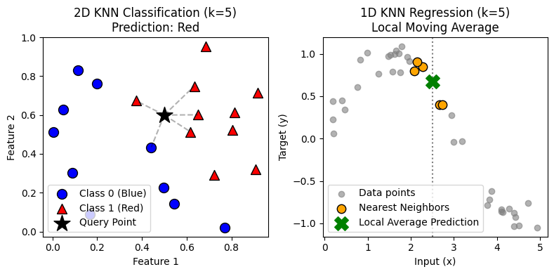
The Regression Process:
Now imagine the marbles aren’t colored, but each has a number written on it (e.g., house price).
- Find the Neighbors: Same as before, identifying the $k$ closest marbles.
- Average: You take the numbers on those 5 marbles—[$200k, $220k, $190k, …]—and calculate their average.
- Predict: That average is your prediction for the new marble.
1.2 The “Smoothing” Knob (k)
 The parameter $k$ controls the “resolution” of your worldview. It represents the trade-off between trusting local data and trusting the general trend.
- Low $k$ (e.g., $k=1$): The Over-Reactor.
- Analogy: You ask only your single closest friend for advice. If they are having a bad day (an outlier), you get bad advice. The decision boundary acts like a jagged coastline, hugging every single data point.
- Technically: Low Bias, High Variance (Overfitting).
- High $k$ (e.g., $k=100$): The Conformist.
- Analogy: You ask 100 people. The unique, nuanced opinions get drowned out by the generic opinion of the masses. The decision boundary becomes a smooth, simple curve that ignores local details.
- Technically: High Bias, Low Variance (Underfitting).
1.3 Why KNN Matters
Even in the age of Deep Learning, KNN concepts are omnipresent.
- Strong Baseline: KNN acts as the perfect “sanity check.” If your complex neural network cannot beat a simple KNN, you are likely overfitting or have bad data.
- Non-Parametric Flexibility: It makes no assumptions about the underlying data distribution (unlike Linear Regression which assumes linearity). It adapts to complex, non-linear decision boundaries.
- Explainability: You can explain any prediction to a non-technical user: “We recommended this product because it is similar to these 5 products you bought.”
- The Backbone of Modern AI: Believe it or not, the most advanced AI systems today—RAG (Retrieval-Augmented Generation)—are essentially giant, turbocharged KNNs. They convert text into vectors and use Approximate Nearest Neighbors (ANN) to find relevant context for the LLM.
2. The Geometry of Similarity
The success of KNN depends almost entirely on how you define “similar.” In machine learning, similarity is the inverse of distance.
2.1 The “Distance” Assumption (Inductive Bias)
If you treat a person’s Age (range 0-100) and Income (range 0-1,000,000) as raw numbers in Euclidean space, distance will be dominated entirely by Income. A difference of 10 years in age ($10^2 = 100$) is negligible compared to a difference of \$100 in income ($100^2 = 10,000$).
Key Insight: KNN is effectively broken without feature scaling (standardization). By scaling features, you are implicitly forcing the “ruler” to treat one unit of Age as equivalent to one unit of standard deviation in Income.
2.2 Distance Metrics: The Math
Let our dataset be $\mathcal{D} = {(\mathbf{x}_i, y_i)}_{i=1}^N$, where $\mathbf{x} \in \mathbb{R}^d$.
The distance between a query $\mathbf{x}$ and a training sample $\mathbf{x}’$ is strictly defined by the Minkowski Distance, which is a generalization of both Euclidean and Manhattan distances:
$$
d_p(\mathbf{x}, \mathbf{x}’) = \left(\sum_{j=1}^{d} |x_j – x’_j|^p\right)^{1/p}
$$
- $p=2$ (Euclidean Distance): “As the crow flies.”
- This is the standard straight-line distance. It works well when features are naturally correlated and represent “spatial” dimensions.
- Default choice for continuous, dense data.
- $p=1$ (Manhattan/Taxicab Distance): “As the cab driver drives.”
- This sums absolute differences. Imagine a grid-like city where you can only move North/South or East/West.
- Why use it? In very high-dimensional spaces (d > 20), Euclidean distance becomes less meaningful because the volume of the space grows exponentially ($r^d$). Manhattan distance is often more robust to outliers because it doesn’t square the error terms, preventing large noise in one dimension from dominating the calculation.
2.3 Cosine Similarity: When Magnitude Doesn’t Matter
In text analysis, two documents might be “similar” because they share topics, even if one is 100 words and the other is 10,000 words. Euclidean distance would penalize the length difference. Cosine similarity looks at the angle between vectors, ignoring their magnitude.
$$
\text{cosine}(\mathbf{x}, \mathbf{x}’) = \frac{\mathbf{x} \cdot \mathbf{x}’}{|\mathbf{x}| |\mathbf{x}’|}
$$
Pro-Tip: If you $\ell_2$-normalize your vectors first (so $|\mathbf{x}|=1$), Euclidean distance and Cosine distance become monotonic to each other.
$$ |\mathbf{x} – \mathbf{x}’|^2 = 2 (1 – \text{cosine}(\mathbf{x}, \mathbf{x}’)) $$
This means you can use optimized libraries that only support Euclidean distance (like some KD-trees) to perform Cosine search, simply by normalizing your data first.
2.4 Distances for Sparse, Binary, and Mixed-Type Features
The “best” distance is rarely universal; it should match how similarity is expressed in your features.
- Binary sets (multi-hot tags): Jaccard distance is often more meaningful than Euclidean distance.
- One-hot categoricals: cosine distance can behave sensibly in high-dimensional sparse spaces.
- Mixed numeric + categorical data: a common pragmatic approach is (i) one-hot encode categoricals, (ii) scale numeric features, and (iii) validate the choice of metric ($p=1$ vs $p=2$, cosine) by cross-validation.
If mixed-type distance is central to the task, consider a dedicated mixed-type dissimilarity (for example, Gower-style distances). In many ML pipelines, however, encoding plus a validated metric is sufficient.
3. The Algorithm: Probability and Aggregation
Once we find the set $\mathcal{N}_k(\mathbf{x})$ of the $k$ nearest neighbors, how do we combine them?
3.1 Classification (The Vote)
We estimate the probability that query $\mathbf{x}$ belongs to class $c$:
$$
P(y=c | \mathbf{x}) = \frac{1}{k} \sum_{i \in \mathcal{N}_k(\mathbf{x})} \mathbb{1}(y_i = c)
$$
The predicted class is simply the argmax of this probability.
Weighted Voting: It is intuitive that a neighbor distance 0.1 away should count more than a neighbor distance 1.0 away. We can weight the vote by the inverse distance $w_i = \frac{1}{d(\mathbf{x}, \mathbf{x}_i)}$.
$$
P(y=c | \mathbf{x}) \propto \sum_{i \in \mathcal{N}_k(\mathbf{x})} w_i \cdot \mathbb{1}(y_i = c)
$$
3.2 Regression (The Average)
Unweighted Mean
$$
\hat{y}(\mathbf{x}) = \frac{1}{k} \sum_{i \in \mathcal{N}_k(\mathbf{x})} y_i
$$
Weighted Mean
$$
\hat{y}(\mathbf{x}) = \frac{\sum_{i \in \mathcal{N}_k(\mathbf{x})} w_i(\mathbf{x})\,y_i}{\sum_{i \in \mathcal{N}_k(\mathbf{x})} w_i(\mathbf{x})}
$$
This weighted form highlights an important connection: KNN regression is a local averaging estimator. With distance-based weights, it resembles kernel regression, where $k$ (and the weights) determine how wide the local neighborhood is.
4. The Curse of Dimensionality (The Silent Killer)
This is the most critical theoretical concept to understand about KNN.
KNN works beautifully in 2D or 3D. But as the number of features (dimensions) $d$ grows (e.g., $d > 20$), something strange happens: intuitions about “space” and “neighbors” break down.
- Empty Space: High-dimensional space is incredibly sparse. To capture $k$ neighbors in 2D, you might need a small circle. To capture the same fraction of data in 100D, you need a hypersphere that touches the very edges of your data boundaries. The “neighborhood” is no longer local; it encompasses most of the dataset.
- Distance Concentration: In very high dimensions, the distance to the nearest neighbor approaches the distance to the farthest neighbor. All points become roughly equidistant from each other.
$$
\lim_{d \to \infty} \frac{\text{dist}_{max} – \text{dist}_{min}}{\text{dist}_{min}} \to 0
$$
The Implication: If you feed 1,000 raw features into KNN, the algorithm is effectively guessing. The distances to all points become roughly the same, indistinguishable from noise.
The Fix: You must reduce dimensions.
- Feature Selection: Use domain knowledge to pick the top 5-10 features.
- Dimensionality Reduction: Use PCA, t-SNE, or UMAP to project data into a lower-dimensional space where Euclidean distance is meaningful again.
5. Computational Reality: $O(N)$ vs $O(\log N)$
KNN is a “Lazy Learner,” meaning training is free (just store the data), but prediction is expensive.
- Training: store $\mathcal{D} = {(\mathbf{x}_i, y_i)}_{i=1}^N$.
- Prediction: for each query point, compute distances to all stored points, pick the closest $k$, aggregate.
The computational and memory cost of prediction would be:
- Brute Force: Calculate distance to all $N$ points. Complexity: $O(N \cdot d)$. This is fine for $N < 10,000$.
- In addition, neighbor selection is $O(N)$ for each query. Also, memory cost is $O(N \cdot d)$ to store the dataset.
- Tree Structures (KD-Trees, Ball Trees): These partition the space into hierarchal boxes. We can ignore whole branches of the tree if we know the query point is far away. Complexity: $O(\log N)$.
- Gotcha: Trees stop working well when $d > 20$. They devolve into Brute Force due to the Curse of Dimensionality.
- Approximate Nearest Neighbors (ANN): For modern RAG (Retrieval Augmented Generation) and search systems with millions of embeddings, we give up “exact” neighbors for “good enough” neighbors using graphs (HNSW) or quantization (FAISS). This brings speed back to milliseconds.
6. Implementation Steps (Practical Checklist)
6.1 Data Preparation
- Define features and target: $\mathbf{X}$ and $\mathbf{y}$.
- Handle missing values: impute or remove.
- Encode categoricals: one-hot encoding is common.
- Scale numeric features: standardize, normalize, or use a robust scaler.
If you have both numeric and categorical features, treat preprocessing as part of the model. In scikit-learn, this typically means a ColumnTransformer inside a Pipeline so that cross-validation does not leak information.
6.2 Model Selection
How do you choose the right hyperparameters?
- Distance Metric: Start with Euclidean ($p=2$). If you have high dimensions ($d > 20$), try Manhattan ($p=1$) or Cosine (if magnitude is irrelevant).
- Choosing $k$:
- Rule of Thumb: A common starting point is $k \approx \sqrt{N}$, where $N$ is the number of samples. This often balances bias and variance reasonably well.
- Tie-Breaking: For binary classification, choose an odd $k$ to avoid 50/50 vote ties.
- Grid Search: Ultimately, $k$ is a hyperparameter you must tune. Plot the error rate on a validation set as you vary $k$ from 1 to 50. You will typically see a “U-shape” curve; the minimum is your optimal $k$.
- Weights: “Distance” weighting is usually superior to “Uniform” because it inherently handles the issue where a distant neighbor has the same voting power as a very close one.
6.3 Evaluation
- Use a train/validation split or cross-validation.
- Use the right metric:
- Classification: accuracy, F1, ROC-AUC, PR-AUC (for imbalance)
- Regression: MAE, RMSE, $R^2$
- Validate that preprocessing is inside a pipeline to avoid leakage.
7. KNN in Python (scikit-learn)
The most robust way to use KNN is as a pipeline: scaling (and other preprocessing) must be learned only from the training folds.
7.1 A Realistic Pattern: Mixed Numeric + Categorical Features
Many real datasets have both numeric and categorical columns. The pattern below keeps preprocessing leakage-safe and makes the “distance geometry” explicit.
from sklearn.compose import ColumnTransformer
from sklearn.impute import SimpleImputer
from sklearn.neighbors import KNeighborsClassifier
from sklearn.pipeline import Pipeline
from sklearn.preprocessing import OneHotEncoder, StandardScaler


numeric_features = ["age", "income"]
categorical_features = ["city", "device"]

numeric_pipe = Pipeline([
    ("imputer", SimpleImputer(strategy="median")),
    ("scaler", StandardScaler()),
])

categorical_pipe = Pipeline([
    ("imputer", SimpleImputer(strategy="most_frequent")),
    ("onehot", OneHotEncoder(handle_unknown="ignore")),
])

preprocess = ColumnTransformer([
    ("num", numeric_pipe, numeric_features),
    ("cat", categorical_pipe, categorical_features),
])

model = Pipeline([
    ("prep", preprocess),
    ("knn", KNeighborsClassifier(n_neighbors=15, weights="distance")),
])If one-hot encoding produces an extremely high-dimensional sparse matrix, validate cosine distance (via metric="cosine" in NearestNeighbors workflows) or consider learning an embedding representation that makes distance meaningful.
A small practical note: many non-Euclidean metrics (including cosine) push scikit-learn toward algorithm="brute". That is often acceptable for small-to-medium datasets, but for larger datasets it is a strong signal that you should consider approximate nearest neighbor indexing.
7.2 Classification Example with Grid Search
import numpy as np

from sklearn.datasets import load_breast_cancer
from sklearn.model_selection import GridSearchCV, train_test_split
from sklearn.neighbors import KNeighborsClassifier
from sklearn.pipeline import Pipeline
from sklearn.preprocessing import StandardScaler
from sklearn.metrics import classification_report


X, y = load_breast_cancer(return_X_y=True)

X_train, X_test, y_train, y_test = train_test_split(
    X, y, test_size=0.2, random_state=42, stratify=y
)

pipe = Pipeline([
    ("scaler", StandardScaler()),
    ("knn", KNeighborsClassifier())
])

param_grid = {
    "knn__n_neighbors": [3, 5, 7, 11, 21],
    "knn__weights": ["uniform", "distance"],
    "knn__p": [1, 2],  # 1=Manhattan, 2=Euclidean for Minkowski
}

search = GridSearchCV(
    pipe,
    param_grid=param_grid,
    cv=5,
    n_jobs=-1,
    scoring="f1"
)

search.fit(X_train, y_train)
print("Best params:", search.best_params_)
print("Best CV score:", search.best_score_)

y_pred = search.predict(X_test)
print(classification_report(y_test, y_pred))7.3 Regression Example (Conceptually Similar)
from sklearn.datasets import load_diabetes
from sklearn.metrics import mean_absolute_error
from sklearn.model_selection import train_test_split
from sklearn.neighbors import KNeighborsRegressor
from sklearn.pipeline import Pipeline
from sklearn.preprocessing import StandardScaler


X, y = load_diabetes(return_X_y=True)

X_train, X_test, y_train, y_test = train_test_split(
    X, y, test_size=0.2, random_state=42
)

model = Pipeline([
    ("scaler", StandardScaler()),
    ("knn", KNeighborsRegressor(n_neighbors=15, weights="distance", p=2))
])

model.fit(X_train, y_train)
pred = model.predict(X_test)
print("MAE:", mean_absolute_error(y_test, pred))8. KNN From Scratch (NumPy-Only, Educational)
This implementation emphasizes the mechanics. It is not intended to be fast.
8.1 Distance Computation: The Vectorization Trick
Naive implementations use nested loops to compute distances, which is painfully slow in Python. A classic linear algebra trick allows us to use matrix multiplication (BLAS) to compute all pairwise distances at once.
We use the identity $(a – b)^2 = a^2 + b^2 – 2ab$. Applied to vectors:
$|\mathbf{x} – \mathbf{y}|^2 = |\mathbf{x}|^2 + |\mathbf{y}|^2 – 2 \mathbf{x} \cdot \mathbf{y}$.
This replaces the slow loop with a fast dot product (@ operator).
import numpy as np

def pairwise_euclidean_distances(X_query: np.ndarray, X_train: np.ndarray) -> np.ndarray:
    """Compute an (n_query, n_train) matrix of Euclidean distances."""
    # (x - y)^2 = x^2 + y^2 - 2xy
    Xq2 = np.sum(X_query ** 2, axis=1, keepdims=True)      # (n_query, 1)
    Xt2 = np.sum(X_train ** 2, axis=1, keepdims=True).T   # (1, n_train)
    cross = X_query @ X_train.T                           # (n_query, n_train)
    d2 = np.maximum(Xq2 + Xt2 - 2.0 * cross, 0.0)
return np.sqrt(d2)8.2 KNN Classification
A note on np.argpartition: We do not need to sort the entire array of distances (which costs $O(N \log N)$). We only need the top $k$. argpartition performs a partial sort in $O(N)$ time, placing the smallest $k$ elements at the beginning (in arbitrary order).
import numpy as np

def knn_predict_class(
    X_train: np.ndarray,
    y_train: np.ndarray,
    X_query: np.ndarray,
    k: int = 5,
    weights: str = "uniform",
    eps: float = 1e-12,
):
    """Educational KNN classifier with deterministic tie-breaking.

    Tie-breaking rule:
    1) Prefer the class with the largest total vote weight.
    2) If tied, prefer the class with the smallest average neighbor distance.
    3) If still tied, prefer the smallest class label.
    """
    distances = pairwise_euclidean_distances(X_query, X_train)  # (n_query, n_train)
    nn_idx = np.argpartition(distances, kth=k - 1, axis=1)[:, :k]  # (n_query, k)

    preds = np.empty(X_query.shape[0], dtype=y_train.dtype)
    for qi, idx in enumerate(nn_idx):
        d = distances[qi, idx]
        y = y_train[idx]

        if weights == "distance":
            w = 1.0 / (d + eps)
        elif weights == "uniform":
            w = np.ones_like(d)
        else:
            raise ValueError("weights must be 'uniform' or 'distance'")

        # Aggregate vote weights per class.
        classes = np.unique(y)
        class_weight = {c: float(np.sum(w[y == c])) for c in classes}
        max_weight = max(class_weight.values())
        tied = [c for c in classes if np.isclose(class_weight[c], max_weight)]

        if len(tied) == 1:
            preds[qi] = tied[0]
            continue

        # Tie-break by smallest average distance among tied classes.
        avg_dist = {c: float(np.mean(d[y == c])) for c in tied}
        min_avg = min(avg_dist.values())
        tied_2 = [c for c in tied if np.isclose(avg_dist[c], min_avg)]
        preds[qi] = min(tied_2)

    return preds
# Define a query point
example_query = np.array([[0.6, 0.4]])

# Run prediction
custom_pred = knn_predict_class(
    X_train=X_class,
    y_train=y_class,
    X_query=example_query,
    k=5,
    weights='uniform'
)

print(f"Query Point: {example_query.tolist()}")
print(f"Predicted Class: {custom_pred[0]}")
# Expected Output:
#     Query Point: [[0.6, 0.4]]
# Predicted Class: 0In practice, distance weighting (weights="distance") is often the simplest way to reduce ties and make predictions smoother near decision boundaries.
8.3 KNN Regression
import numpy as np

def knn_predict_regression(
	X_train: np.ndarray,
	y_train: np.ndarray,
	X_query: np.ndarray,
	k: int = 5,
	weights: str = "uniform",
	eps: float = 1e-12,
):
	"""Educational KNN regressor (unweighted or distance-weighted)."""
	distances = pairwise_euclidean_distances(X_query, X_train)  # (n_query, n_train)
	nn_idx = np.argpartition(distances, kth=k - 1, axis=1)[:, :k]  # (n_query, k)

	preds = np.empty(X_query.shape[0], dtype=float)
	for qi, idx in enumerate(nn_idx):
		d = distances[qi, idx]
		y = y_train[idx].astype(float)

		if weights == "distance":
			w = 1.0 / (d + eps)
			preds[qi] = float(np.sum(w * y) / np.sum(w))
		elif weights == "uniform":
			preds[qi] = float(np.mean(y))
		else:
			raise ValueError("weights must be 'uniform' or 'distance'")

	return preds

# Define a query point (must be 2D for the pairwise distance function)
query_x = np.array([[2.5]])

# Run prediction
custom_reg_pred = knn_predict_regression(
    X_train=X_reg,
    y_train=y_reg,
    X_query=query_x,
    k=5,
    weights='uniform'
)

print(f"Query Point (x): {query_x[0][0]}")
print(f"Predicted Value (y): {custom_reg_pred[0]:.4f}")
print(f"Actual Sine Value: {np.sin(2.5):.4f}")
# Expected Output:
#     Query Point (x): 2.5
#     Predicted Value (y): 0.4137
# Actual Sine Value: 0.59859. Practical Tips and Best Practices
9.1 Choosing $k$
- Small $k$ yields low bias but high variance (sensitive to noise).
- Large $k$ yields higher bias but lower variance (smoother boundary).
- A pragmatic approach is to grid-search $k$ and select by cross-validation.
- For binary classification, an odd $k$ can reduce ties in unweighted voting.
For theoretical intuition, it is helpful to remember a classic consistency condition (informal statement): in many standard settings, $k$-NN classification is consistent (its risk approaches the Bayes risk) as data grows if
$$
k \to \infty \quad \text{and} \quad \frac{k}{n} \to 0 \quad \text{as} \quad n \to \infty.
$$
Intuitively, you want neighborhoods to contain more points (to reduce variance) while still shrinking in radius (to keep bias under control).
9.2 Consider Distance-Weighted Neighbors
weights="distance"often helps when the nearest points are much closer than the rest.- Distance weighting can reduce sensitivity to the exact choice of $k$.
9.3 Handle Class Imbalance Explicitly
- Use evaluation metrics that reflect the business objective (F1, PR-AUC).
- Consider distance weighting and careful thresholding (for probabilistic outputs).
- Inspect confusion matrices and per-class metrics.
9.4 Fast Inference: Use the Right Backend
- For small datasets, brute force is acceptable.
- For moderate datasets, KD-tree/Ball-tree can help.
- For large-scale retrieval, approximate nearest neighbor indexing is often the practical choice.
9.5 Probability Outputs and Calibration
KNeighborsClassifier can output class probabilities via predict_proba(), typically as neighbor vote fractions (or distance-weighted fractions). These “probabilities” are often useful for ranking, but they are not guaranteed to be well-calibrated.
Practical guidance:
- If probability calibration matters (for example, decision thresholds or risk estimates), consider calibration methods (Platt scaling or isotonic regression) on a validation set.
- If you change preprocessing or $k$, re-check calibration; it can shift noticeably.
Common Failure Modes (Debugging Checklist)
- Accuracy is unexpectedly low: check scaling, metric choice, and feature leakage.
- Model is slow at inference: reduce $n$, reduce $d$, use an index, or use ANN.
- Overfitting (great train, poor test): increase $k$, add regularizing preprocessing (PCA), remove noisy features.
- Underfitting (poor everywhere): decrease $k$, improve feature engineering, or change distance metric.
- Sensitive to one feature: verify scaling and consider robust scaling.
- Unexpected train–test gap after cross-validation: verify that all preprocessing (imputation, scaling, PCA) is inside a single pipeline.
Summary
KNN is more than just a classification algorithm; it is a fundamental way of thinking about data. It teaches us that “intelligence” often boils down to two things:
- Memory: Storing past experiences.
- Similarity: Knowing which past experience is relevant to use right now.
While simplistic in execution, the principles of KNN underly everything from Netflix recommendations to Spotify playlists and modern RAG systems.
Key Takeaways
- Geometry is Everything: Preprocessing (scaling) and metric selection (Euclidean vs Cosine) dictate performance.
- Beware the Curse: In high dimensions ($d > 20$), distance loses meaning. Reduce dimensions first.
- Tune $k$: It’s your smoothing knob. Low $k$ overfits; high $k$ underfits.
When KNN Shines
- Explainability First: When you need to show users “why” (e.g., “People like you also bought…”).
- Small, Clean Data: $N < 100k$, features < 20.
- Complex Decision Boundaries: When linear models fail to capture the wiggly nature of the real world.
- Strong Baselines: Always run KNN before training a Neural Network.
When KNN Struggles
- High Latency Requirements: If you need $<10ms$ predictions on millions of rows without ANN.
- High Dimensions: Raw images, raw audio.
- Sparse Data: High-dimensional sparse matrices (unless using Cosine distance carefully).
- Outliers: Especially with low $k$, a single wrong data point can create an island of false predictions.

Happy is a seasoned ML professional with over 15 years of experience. His expertise spans various domains, including Computer Vision, Natural Language Processing (NLP), and Time Series analysis. He holds a PhD in Machine Learning from IIT Kharagpur and has furthered his research with postdoctoral experience at INRIA-Sophia Antipolis, France. Happy has a proven track record of delivering impactful ML solutions to clients.

Silpa brings 5 years of experience in working on diverse ML projects, specializing in designing end-to-end ML systems tailored for real-time applications. Her background in statistics (Bachelor of Technology) provides a strong foundation for her work in the field. Silpa is also the driving force behind the development of the content you find on this site.
Subscribe to our newsletter!