Before LightGBM entered the scene, another algorithm reigned supreme in the world of machine learning competitions and industrial applications: XGBoost.
XGBoost (short for eXtreme Gradient Boosting) is the workhorse of tabular machine learning: fast, regularized, and remarkably reliable across a wide range of datasets.
If you picture gradient boosting as a team of small decision trees taking turns to correct each other’s mistakes, XGBoost is that same team with:
- a smarter training signal (it uses both gradient and curvature),
- guardrails against overfitting (regularization + conservative splitting), and
- system optimization (parallel tree building, efficient split search, sparsity awareness, automatic missing value handling, and optional GPU support).
In this article, we will peel back the layers of XGBoost. We will start with the high-level intuition, dive deep into the second-order calculus that makes it “extreme,” and finally look at how to tune it like a pro.
This article is organized into 5 parts:
- Foundations of Boosting
- XGBoost Algorithm in Depth
- Hyperparameters & Tuning Strategy
- Practical Implementation & Interpretation
- Advanced Topics, Ecosystem, and Comparisons
Part 1: Foundations of Boosting & Gradient Boosting Machines
Ensemble Learning
Ensembles combine multiple weak (or diverse) learners to form a strong predictor. Two broad paradigms:
- Bagging (parallel aggregation; reduces variance) — e.g. Random Forest.
- Boosting (sequential correction; reduces bias while controlling variance) — each new model focuses on previous errors.
Think of Boosting like a game of golf.
- The Tee Shot (The First Model): You hit the ball towards the hole (the target). You probably won’t get a hole-in-one. The ball lands somewhere on the fairway.
- The Approach Shot (The Second Model): You don’t go back to the tee. You walk to where the ball landed. Your goal now is to hit the ball the remaining distance to the hole (the residual).
- The Putt (The Third Model): You are close now. You just need a small nudge to correct the remaining error.
In boosting, each “shot” is a decision tree. The first tree predicts the target. The second tree predicts the error of the first tree. The third tree predicts the error of the combined first and second trees. When you add them all up, you get to the hole.
Gradient Boosting Machines: Core Mechanics
Boosting starts with a base prediction (often a constant, like the average of the targets) and iteratively adds weak learners that minimize the current loss. Each new expert (often a small decision tree) corrects the most obvious errors, then the next expert focuses on the remaining errors, and so on.
For a dataset with $n$ samples $(x_i, y_i)$, the goal is to learn a function $F(x)$ that minimizes a differentiable loss function $l(y, \hat{y})$ using $K$ additive functions (weak learners; e.g., decision trees):
$$\hat{y_i} = F(x_i) = \sum_{k=1}^{K} f_k(x_i)$$
Thus, the objective is:
$$ \mathcal{L} = \sum_{i=1}^{n} l(y_i, F(x_i)) $$
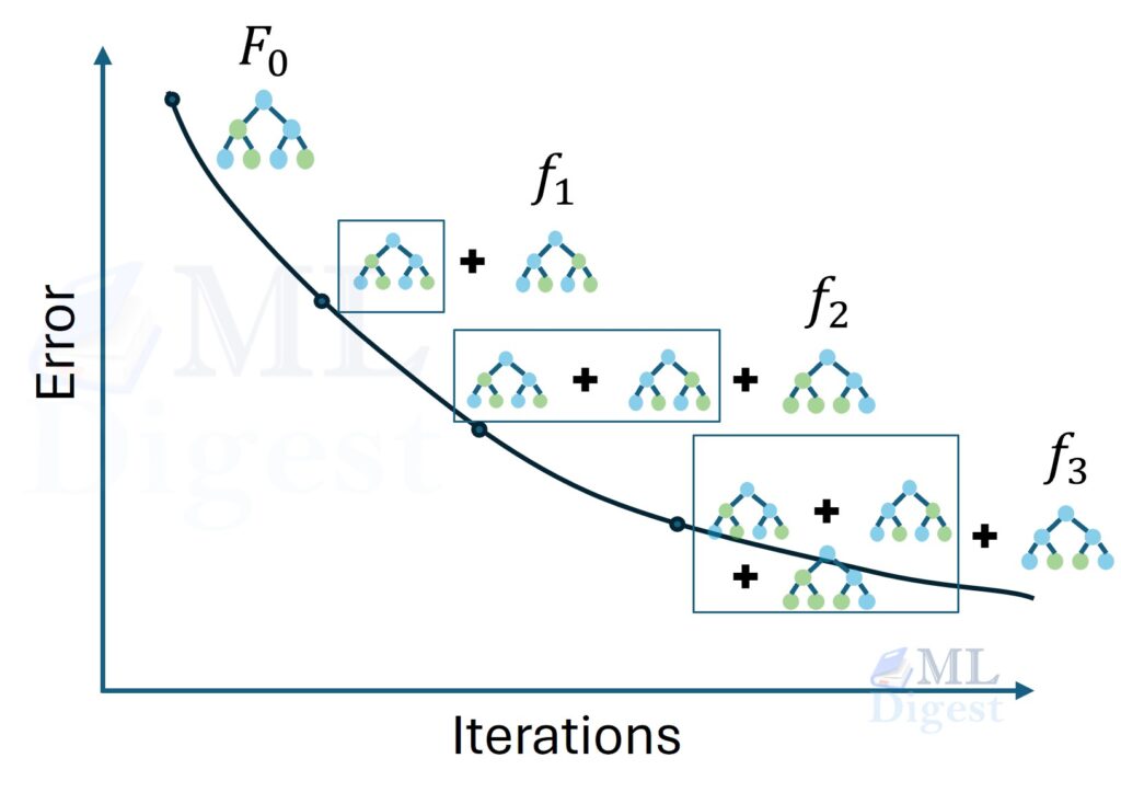
The model is built in stages. At each stage $k$, we add a new function $f_k$ to the existing ensemble $F_{k-1}$:
$$F_k(x_i) = F_{k-1}(x_i) + \eta f_k(x_i)$$
where $\eta$ is the learning rate (shrinkage). Think of $\eta$ as the “step size” in our golf analogy. We don’t want to hit the ball 100% of the distance the model suggests, because the model might be overfitting to noise. We take a small step (e.g., 0.1) in the right direction.
So at each iteration $k$, the model aims to minimize the overall loss function $l(y, \hat{y})$ (e.g., squared error for regression, logistic loss for classification), and the objective funstion can be represented as:
$$ \begin{align} \mathcal{L} &= \sum_{i=1}^{n} l(y_i, F_k(x_i)) \\ &= \sum_{i=1}^{n} l\left(y_i, F_{k-1}(x_i) + \eta f_k(x_i)\right) \end{align}$$
Gradient Descent in Function Space:
This is the “Aha!” moment for Gradient Boosting. In standard Gradient Descent (like in Neural Networks), we update the parameters (weights) of the model to minimize loss. In Gradient Boosting, we update the function itself.
At each iteration $k$, we calculate the pseudo-residuals ($r_i^{(k)}$), which are simply the negative gradients of the loss function with respect to the current predictions:
$$
r_i^{(k)} = – \left. \frac{\partial l(y_i, F_{k-1}(x_i))}{\partial F_{k-1}(x_i)} \right.
$$
If the loss function is Squared Error (MSE), the negative gradient is exactly $(y_i – \hat{y}_i)$—the literal residual. If the loss function is Log Loss, the gradient is the difference between the probability and the label.
In essence, each new weak learner $f_k$ is trained to predict these pseudo-residuals. The updated model after $K$ iterations can be expressed as:
$$F_K(x) = F_0(x) + \sum_{k=1}^{K} \eta\, f_k(x)$$
where $F_0(x)$ is the initial prediction (e.g., mean target).
This can be simplified further to obtain the first equation:
$$\hat{y_i} = F_K(x) = \sum_{k=1}^{K} f_k(x)$$
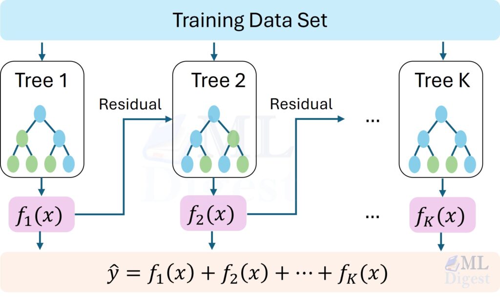
In gradient boosting, each new tree is trained to predict these pseudo-residuals. XGBoost goes further, using both the gradient and the curvature (second-order, or Hessian, information) for smarter, more stable updates. Thus, XGBoost supercharges this concept, correcting errors efficiently and robustly, with built-in safeguards against overfitting. Visit here for more details.
Brief look at AdaBoost: It adjusts sample weights so misclassified points get higher weight. Uses exponential loss; sensitive to noisy labels but elegant. Gradient boosting generalizes this: instead of reweighting examples, it fits gradients of any differentiable loss.
Limitations of Standard GBM:
- Slower for large data (exact split scan costs)
- Limited regularization (risk of overfitting)
- Weak native handling of missing values
- No integrated second-order optimization
XGBoost solves or mitigates each.
Part 2: The XGBoost Algorithm — Objective, Optimization, and Tree Building
What Makes XGBoost “Extreme”?
XGBoost isn’t just “Gradient Boosting with a cool name.” It introduces three key innovations:
- Regularized Objective: It penalizes complex trees to prevent overfitting.
- Second-Order Approximation: It uses the Hessian (curvature) to make smarter updates.
- System Optimizations: It is engineered for speed (block structure, cache awareness, out-of-core computing).
Let’s break down the math, starting with the objective function.
The Regularized Objective Function
XGBoost minimizes a more sophisticated objective function than traditional gradient boosting:
$$\begin{align} \mathcal{L} &= \sum_{i=1}^{n} l\big(y_i, \hat{y}i\big) + \sum_{k=1}^{K} \Omega(f_k) \\
&= \sum_{i=1}^{n} l\big(y_i, F_{k-1}(x_i) + \eta f_k(x_i)\big) + \sum_{k=1}^{K} \Omega(f_k)
\end{align}$$
Where $l(y_i, \hat{y}_i)$ is the loss (e.g., logistic loss, squared error), and $\Omega(f_k)$ penalizes the complexity of tree $f_k$.
A common tree penalty is:
$$
\Omega(f) = \gamma T + \frac{1}{2} \lambda \sum_{j=1}^{T} w_j^2
$$
Here:
- $T$ is the number of leaves.
- $w_j$ is the score (weight) of leaf $j$.
- $\gamma$ (gamma) is the penalty for adding a new leaf.
- $\lambda$ (lambda) is the L2 regularization term on the weights.
The key idea is simple: a split must earn its keep. It’s not enough to just lower the training error; the improvement must be large enough to offset the penalty ($\gamma$) of adding a new branch. Regularization includes an $L_2$ penalty by default and can include $L_1$ as well.
System Optimizations:
- Columnar block structure for efficient scanning
- Cache-aware memory access
- Parallel split evaluation (CPU threads; GPU kernels)
- Weighted Quantile Sketch for large/sparse data
- Distributed training support
Mathematical Formulation: The Taylor Expansion Trick
At iteration $k$, we want to find a tree $f_k$ that minimizes:
$$\mathcal{L}^{(k)} = \sum_{i=1}^n l\big(y_i, F_{k-1}(x_i) + f_k(x_i)\big) + \Omega(f_k)$$
Optimizing a general loss function (like Log Loss) directly for a tree structure is hard. The function is complex and non-linear.
XGBoost uses a Second-Order Taylor Expansion to approximate the loss function with a parabola (a quadratic equation). Why? Because quadratic equations are easy to minimize—we know exactly where the bottom of the curve is.
Taylor Expansion of Loss:
We approximate the loss around the current prediction $F_{k-1}(x_i)$:
$$l(y_i, F_{k-1}(x_i) + f_k(x_i)) \approx l(y_i, F_{k-1}(x_i)) + g_i f_k(x_i) + \frac{1}{2} h_i f_k(x_i)^2$$
Where $g_i$ and $h_i$ are the first and second derivatives (gradient and Hessian) of the loss.
$$g_i = \left. \frac{\partial l(y_i, \hat{y}_i)}{\partial \hat{y}_i} \right|_{\hat{y}_i=F_{k-1}(x_i)},\quad h_i = \left. \frac{\partial^2 l(y_i, \hat{y}_i)}{\partial \hat{y}_i^2} \right|_{\hat{y}_i=F_{k-1}(x_i)}$$
- Gradient ($g_i$): The direction we should move.
- Hessian ($h_i$): How “confident” we should be (curvature). If the curvature is high, we are near a minimum, so we should take smaller steps.
Simplified Objective:
Removing constants, we get a simple quadratic sum:
$$\mathcal{L}^{(k)} \approx \sum_{i=1}^n \big( g_i f_k(x_i) + \frac{1}{2} h_i f_k(x_i)^2 \big) + \Omega(f_k)$$
The Structure Score: How Good is a Tree?
Now, we group the samples by the leaf they end up in. Let $I_j$ be the set of samples in leaf $j$, then $f_k(x_i)=w_j$.
Group by leaves ($I_j$ index set):
$$\mathcal{L}^{(k)} = \sum_{j=1}^T \Big( \sum_{i \in I_j} g_i w_j + \frac{1}{2} \sum_{i \in I_j} h_i w_j^2 \Big) + \gamma T + \frac{1}{2}\lambda \sum_{j=1}^T w_j^2$$
We define $G_j = \sum_{i \in I_j} g_i$ (sum of gradients in leaf $j$) and $H_j = \sum_{i \in I_j} h_i$ (sum of hessians in leaf $j$), thus:
$$\mathcal{L}^{(k)} = \sum_{j=1}^T \Big( G_j w_j + \frac{1}{2} (H_j + \lambda) w_j^2 \Big) + \gamma T$$
The optimal weight $w_j^*$ for leaf $j$ is: $$w_j^* = – \frac{G_j}{H_j + \lambda}$$
And the quality (score) of that leaf structure is:
$$\text{Score}(j) = -\frac{1}{2} \frac{G_j^2}{H_j + \lambda} + \gamma$$
Intuition:
- $G_j^2$: We want the gradients in a leaf to be large (meaning we are correcting a big error).
- $H_j + \lambda$: We divide by the Hessian (plus regularization). If the curvature is high (or we regularize heavily), the score decreases.
Split Gain:
When deciding whether to split a node $(G,H)$ into left $(G_L,H_L)$ and right $(G_R,H_R)$, XGBoost calculates the Gain:
$$\text{Gain} = \frac{1}{2} \left( \underbrace{\frac{G_L^2}{H_L + \lambda}}_\text{score of left child} + \underbrace{\frac{G_R^2}{H_R + \lambda}}_\text{score of right child} – \underbrace{\frac{G^2}{H + \lambda}}_\text{score if not splitted} \right) – \underbrace{\gamma}_\text{Complexity penalty}
$$
If Gain > 0, the split is worth it. If Gain < 0, the split doesn’t improve the model enough to justify the added complexity ($\gamma$), so we don’t split (or we prune it later).
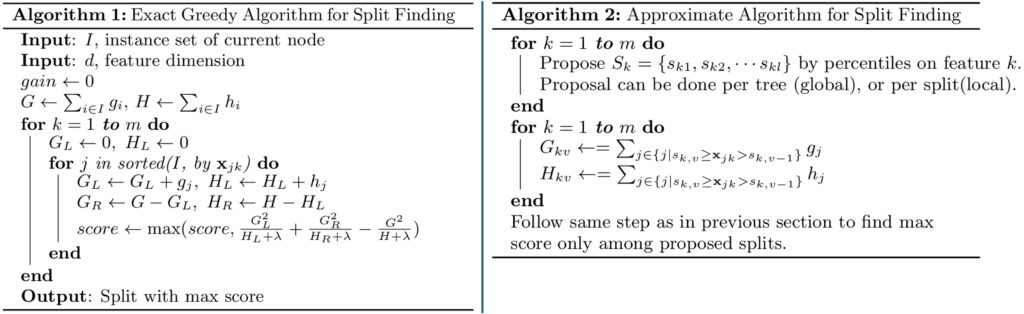
Tree Building & Splitting:
- Exact Greedy Algorithm: For small data, it scans every possible split point.
- Approximate Algorithm (Histogram): For large data, it bins continuous features into buckets (histograms) and only checks split points at the bucket boundaries.
- Sparsity-Awareness: XGBoost learns a “default direction” for missing values. If a value is missing, it goes left or right depending on which direction minimizes loss.
Boosters Beyond Trees:
- Linear Booster (
gblinear): regularized linear model for high-dimensional, mostly linear data - DART Booster (
dart): dropout trees during training for better generalization


Part 3: Hyperparameters, Tuning, and Model Interpretation
Tuning XGBoost can feel like flying a spaceship—there are a lot of buttons. (Full List Here)
1. The “Brakes” (Preventing Overfitting)
These parameters stop the model from memorizing the training data.
max_depth(Default: 6): How deep each tree can grow. Deeper trees capture more complex interactions but are more likely to overfit.- Intuition: A depth of 1 is a “stump” (very simple). A depth of 10 is a complex rule set. Start with 4-6.
min_child_weight(Default: 1): The minimum sum of instance weight (Hessian) needed in a child.- Intuition: If a leaf node represents only a few data points (or points with low confidence), this parameter stops the split. Increase this to make the model more conservative.
gamma(Default: 0): The minimum loss reduction required to make a split.- Intuition: This is the “hurdle” a split must jump over. If the gain is less than
gamma, the split doesn’t happen.
- Intuition: This is the “hurdle” a split must jump over. If the gain is less than
2. The “Steering” (Randomness & Diversity)
These parameters add randomness to make the ensemble robust (similar to Random Forest).
subsample(Default: 1): The fraction of data samples used to train each tree.- Recommendation: Set to 0.7 – 0.9 to prevent overfitting.
colsample_bytree(Default: 1): The fraction of features (columns) used for each tree.- Recommendation: Set to 0.7 – 0.9. This is crucial if you have many correlated features.
3. The “Engine” (Learning Speed)
eta/learning_rate(Default: 0.3): The step size.- Strategy: Usually, you want a lower learning rate (e.g., 0.01 or 0.05) combined with a higher number of trees (
n_estimators). This takes longer to train but usually yields better results.
- Strategy: Usually, you want a lower learning rate (e.g., 0.01 or 0.05) combined with a higher number of trees (
n_estimators(ornum_boost_round): The number of trees to build.- Strategy: Always use Early Stopping. Set
n_estimatorsto a high number (e.g., 1000) and let early stopping find the optimal point.
- Strategy: Always use Early Stopping. Set
4. The “Regularizers” (L1/L2)
lambda(L2 regularization): Smooths the leaf weights. Good for reducing the impact of outliers.alpha(L1 regularization): Encourages sparsity (driving some weights to zero). Useful for high-dimensional data.
Tuning Strategy: The “Control Complexity First” Approach
Don’t just grid search everything at once. Follow this sequence:
- Set a Baseline: Fix
learning_rateto 0.1. - Tune Tree Complexity: Grid search
max_depth(e.g., [3, 5, 7, 9]) andmin_child_weight(e.g., [1, 3, 5]). - Tune Randomness: Grid search
subsampleandcolsample_bytree(e.g., [0.6, 0.8, 1.0]). - Tune Regularization: If still overfitting, try increasing
gamma,lambda, oralpha. - Lower Learning Rate: Once you have good structural parameters, lower the
learning_rate(e.g., to 0.01) and increasen_estimators.
Practical heuristic: if the model overfits early, start by increasing min_child_weight and gamma before touching learning_rate.
Model Interpretation and Essential Features
Early Stopping: Monitor validation metric; stops when no improvement for N rounds.
Handling Categorical Data: Recent XGBoost versions support categorical splits, but the details depend on the API and tree_method. In practice, integer-encode categories and consult the current XGBoost docs for your installed version. If native categorical support is not available or unstable for your setup, one-hot encoding or target encoding is still a strong baseline.
Imbalanced Data: Set scale_pos_weight = (num_negative / num_positive).
Evaluation Metrics:
- Classification:
logloss,auc,error - Regression:
rmse,mae - Ranking:
ndcg,map
Feature Importance:
- Weight: # times feature used in splits
- Gain: Average gain contributed
- Cover: Proportion of samples affected
Part 4: Practical Implementation
DMatrix: Optimized internal data format supporting sparsity & weight handling.
import xgboost as xgb
X_train, y_train = ...  # numpy / pandas
dtrain = xgb.DMatrix(X_train, label=y_train)Training with xgb.train:
params = {
    'objective': 'binary:logistic',
    'eval_metric': 'logloss',
    'eta': 0.1,
    'max_depth': 6,
    'subsample': 0.8,
    'colsample_bytree': 0.8,
}
watchlist = [(dtrain, 'train')]
bst = xgb.train(params, dtrain, num_boost_round=300)Cross-Validation xgb.cv:
cv_res = xgb.cv(
    params,
    dtrain,
    num_boost_round=500,
    nfold=5,
    early_stopping_rounds=30,
    metrics=['logloss'],
    seed=42
)
best_rounds = cv_res.shape[0]Scikit-Learn Wrapper:
from xgboost import XGBClassifier
clf = XGBClassifier(
    objective='binary:logistic',
    eval_metric='logloss',
    n_estimators=500,
    learning_rate=0.05,
    max_depth=6,
    subsample=0.8,
    colsample_bytree=0.8,
    early_stopping_rounds=30
)
clf.fit(X_train, y_train, eval_set=[(X_valid, y_valid)], verbose=False)Full Example (Classification):
import xgboost as xgb
from sklearn.datasets import make_classification
from sklearn.model_selection import train_test_split
from sklearn.metrics import accuracy_score

X, y = make_classification(n_samples=10000, n_features=20, random_state=42)
X_train, X_test, y_train, y_test = train_test_split(X, y, test_size=0.2, random_state=42)

model = xgb.XGBClassifier(
    objective='binary:logistic',
    n_estimators=1000,
    learning_rate=0.03,
    max_depth=6,
    subsample=0.8,
    colsample_bytree=0.8,
    eval_metric='logloss',
    early_stopping_rounds=50
)
model.fit(X_train, y_train, eval_set=[(X_test, y_test)], verbose=False)
preds = model.predict(X_test)
print(f"Accuracy: {accuracy_score(y_test, preds):.4f}")Part 5: Comparisons with Other Ensemble Methods
XGBoost does not exist in a vacuum. While it revolutionized the field, it sits in a landscape between its predecessor (Random Forest) and its modern successors (LightGBM and CatBoost). Understanding the differences is crucial for choosing the right tool for the job.
1. XGBoost vs. Random Forest: Bagging vs. Boosting
The most fundamental comparison is between the two giants of tabular learning.
- The Intuition:
- Random Forest is like a democracy. You ask 100 people for their opinion, and you take the average (or majority vote). The people (trees) are independent; they do not talk to each other. This averages out errors and reduces variance.
- XGBoost is like a relay race or a specialized surgical team. The first member does the broad work. The second member looks at what the first missed and fixes it. The third fixes the remaining small errors. They work sequentially, and each member is aware of the previous member’s mistakes.
- The Technical Difference:
- Random Forest uses Bagging (Bootstrap Aggregating). It builds deep, fully grown trees in parallel on random subsets of data. It has no global objective function it is trying to minimize; it just reduces variance by averaging.
- XGBoost uses Boosting. It builds shallow trees sequentially. It optimizes a specific differentiable loss function using gradient descent in function space.
- Verdict: Use Random Forest for a quick, robust baseline that is hard to overfit. Use XGBoost when you need to squeeze every ounce of performance out of the data and are willing to tune hyperparameters.
2. XGBoost vs. LightGBM: The Battle for Speed
Microsoft released LightGBM in 2017 to solve the scalability issues of XGBoost.
- The Intuition:
- Imagine building a building. XGBoost (historically) builds it floor by floor (Level-wise). It finishes the first floor completely before starting the second. This is safe and stable.
- LightGBM builds the room that needs the most attention first (Leaf-wise). If the kitchen is the most important part, it builds the kitchen, then the pantry, then the stove, potentially ignoring the bedroom for a while. It chases the “loss” aggressively.
- The Technical Difference:
- Growth Strategy: XGBoost defaults to Level-wise growth (symmetric). LightGBM defaults to Leaf-wise (best-first) growth. Leaf-wise is usually faster and achieves lower loss, but it can overfit on small datasets if not constrained (by
max_depth). - Split Finding: LightGBM introduced histogram-based splitting (binning continuous values) to speed up training dramatically. XGBoost later adopted this (via
tree_method='hist'), so the speed gap has narrowed significantly.
- Growth Strategy: XGBoost defaults to Level-wise growth (symmetric). LightGBM defaults to Leaf-wise (best-first) growth. Leaf-wise is usually faster and achieves lower loss, but it can overfit on small datasets if not constrained (by
3. XGBoost vs. CatBoost: The Categorical Specialist
Yandex released CatBoost to handle non-numeric data better.
- The Intuition:
- Most algorithms speak only numbers. If you have a category like “Color: Red”, you have to translate it (One-Hot Encoding).
- CatBoost is a polyglot. It speaks “Category” natively. It uses clever statistics to turn categories into numbers during training without cheating (target leakage).
- The Technical Difference:
- Categorical Handling: CatBoost uses Ordered Target Statistics. It calculates the average target value for a category, but only using “past” data points in a virtual time sequence, preventing the model from seeing the answer before predicting it.
- Symmetric Trees: CatBoost uses “oblivious trees” where the same split condition is applied across the entire level of the tree. This acts as a strong regularizer and enables very fast inference.
Summary Comparison Table
| Feature | XGBoost | Random Forest | LightGBM | CatBoost |
|---|---|---|---|---|
| Core Concept | Gradient Boosting (Sequential correction) | Bagging (Parallel voting) | Gradient Boosting (Leaf-wise growth) | Gradient Boosting (Ordered boosting) |
| Tree Growth | Level-wise (Depth-first). Stable. | Level-wise (Independent). | Leaf-wise (Best-first). Fast, aggressive. | Symmetric. Balanced, fast inference. |
| Categorical Data | Traditionally required encoding. Newer versions support native experimental handling. | Requires encoding (One-Hot/Label). | Native support (Gradient-based). | Best-in-class native support (Ordered TS). |
| Missing Values | Sparsity-aware: Learns default directions. | Requires imputation. | Native handling. | Native handling (Min/Max/Separate). |
| Speed | Fast (especially with hist mode). | Moderate (Parallel but deep trees). | Very Fast (optimized for large data). | Slower training, very fast prediction. |
| Best Use Case | The “All-Rounder”. Kaggle winner. Reliable. | The “Baseline”. Quick, easy, robust. | Massive datasets (>10M rows). | Dirty data with many categories. |
The Decision Guide: Which one should you choose?
- Start with Random Forest if you want a quick answer and do not want to tune parameters.
- Switch to XGBoost if you need higher accuracy or have missing values. It is the industry standard for a reason.
- Use LightGBM if your dataset is massive (millions of rows) and XGBoost is taking too long.
- Use CatBoost if you have many categorical features (strings) and do not want to deal with complex preprocessing or encoding.
Final Summary
XGBoost extends classical GBM with second‑order optimization, strong regularization, efficient split finding, native handling of sparsity, and production-grade scalability. Choose it when:
- You need a reliable tabular baseline
- Interpretability via tree structures + SHAP is required
- Data includes missing values and mixed feature types
- You want stable training across a wide hyperparameter space
If extreme speed with very large datasets is critical, test LightGBM; if categorical handling dominates, evaluate CatBoost. But XGBoost remains the most balanced “all-terrain” framework.
FAQ
When to prefer XGBoost over LightGBM or CatBoost?
When to prefer XGBoost over LightGBM or CatBoost?
XGBoost is a solid all-rounder, especially when interpretability and robustness are priorities. Choose it when:
- You need a reliable tabular baseline.
- Interpretability via tree structures + SHAP is required.
- Data includes missing values and mixed feature types.
- You want stable training across a wide hyperparameter space.
How does XGBoost handle missing values?
How does XGBoost handle missing values?
XGBoost learns a default direction for missing values during split finding. When evaluating splits, it tries sending missing values left and right, choosing the direction that yields higher gain. This allows it to natively handle missing data without explicit imputation.
What Makes XGBoost So Powerful?
What Makes XGBoost So Powerful?
1. Regularization: This is XGBoost’s secret weapon. It adds a penalty term to the objective function (both L1 and L2 regularization) that discourages overly complex models. This helps prevent overfitting and makes the model generalize better to new data.
2. Handling Missing Values: XGBoost has a built-in routine to handle missing data. During training, it learns the best direction to send data points with missing values, making data preprocessing much simpler.
3. Tree Pruning: While traditional gradient boosting stops splitting a node once it hits a negative loss, XGBoost grows the tree to a max_depth and then prunes it backward. It removes splits that don’t provide a positive gain, leading to more robust trees.
4. Parallel Processing: XGBoost can parallelize the construction of trees, making it significantly faster than standard gradient boosting implementations.
5. Cache-Aware Access: XGBoost is designed to make optimal use of hardware. It organizes data in memory to minimize cache misses, speeding up computation.
How does XGBoost differ from traditional Gradient Boosting Machines (GBM)?
How does XGBoost differ from traditional Gradient Boosting Machines (GBM)?
XGBoost enhances traditional GBM in several key ways:
- Second-Order Optimization: XGBoost uses both first and second derivatives (gradients and Hessians) of the loss function for more accurate approximations during tree construction.
- Regularization: It incorporates L1 and L2 regularization directly into the objective function, reducing overfitting.
- Efficient Split Finding: XGBoost employs advanced algorithms like weighted quantile sketching for faster split finding, especially on large datasets.
- Sparsity Awareness: It natively handles missing values and sparse data without requiring explicit imputation.
What are pseudo-residuals in XGBoost?
What are pseudo-residuals in XGBoost?
Pseudo-residuals are the negative gradients of the loss function with respect to the current model’s predictions. At each iteration, XGBoost fits a new tree to these pseudo-residuals, effectively learning how to correct the errors made by the existing ensemble of trees. This approach allows XGBoost to iteratively improve its predictions by focusing on the areas where it is currently underperforming.
Can XGBoost handle categorical features directly?
Can XGBoost handle categorical features directly?
Recent versions of XGBoost support categorical features natively when using the enable_categorical=True flag in the DMatrix. Categorical features should be integer-encoded. However, for older versions or more complex categorical handling, techniques like target encoding or one-hot encoding may still be necessary.
How does XGBoost handle imbalanced datasets?
How does XGBoost handle imbalanced datasets?
XGBoost provides the scale_pos_weight parameter to help manage imbalanced datasets. This parameter adjusts the weight of positive class instances during training, helping to balance the influence of each class on the model’s learning process. A common approach is to set scale_pos_weight to the ratio of negative to positive instances in the dataset.
How does XGBoost implement regularization?
How does XGBoost implement regularization?
XGBoost incorporates regularization directly into its objective function through two main components:
- L1 Regularization (Lasso Regression): This term adds a penalty equal to the absolute value of the magnitude of coefficients. It can lead to sparse models where some feature weights are exactly zero, effectively performing feature selection.
- L2 Regularization (Ridge Regression): This term adds a penalty equal to the square of the magnitude of coefficients. It helps to prevent overfitting by discouraging overly complex models.
By combining these two forms of regularization, XGBoost can produce more robust models that generalize better to unseen data.
How does XGBoost handle missing values?
How does XGBoost handle missing values?
XGBoost has a built-in mechanism to handle missing values during training. When constructing trees, it learns the best direction (left or right) to send instances with missing values at each split. This means that you don’t need to perform any explicit imputation of missing data before training the model, simplifying the preprocessing pipeline.
What are the different tree growth policies in XGBoost?
What are the different tree growth policies in XGBoost?
XGBoost offers two primary tree growth policies:
- Depthwise Growth (default): This policy grows trees level by level, ensuring that all nodes at a given depth are expanded before moving to the next level. This approach tends to create balanced trees.
- Lossguide Growth: This policy grows trees by focusing on the nodes that provide the highest loss reduction, allowing for deeper and potentially more complex trees. This can be beneficial for datasets with high dimensionality or when capturing intricate patterns is necessary.
What are the different boosters available in XGBoost?
What are the different boosters available in XGBoost?
XGBoost provides several booster options to suit different types of problems:
- Tree Booster (
gbtree): The default and most commonly used booster, which builds decision trees for regression and classification tasks. - Linear Booster (
gblinear): Uses linear models instead of trees, suitable for high-dimensional data where linear relationships dominate. - DART Booster (
dart): Implements dropout techniques to randomly drop trees during training, helping to reduce overfitting and improve generalization. - GPU Booster: XGBoost supports GPU acceleration for faster training on large datasets, particularly useful when using the histogram-based tree method.
How does XGBoost implement early stopping?
How does XGBoost implement early stopping?
XGBoost implements early stopping by monitoring a specified evaluation metric on a validation set during training. If the metric does not improve for a defined number of consecutive rounds (specified by the early_stopping_rounds parameter), the training process halts early. This helps prevent overfitting and allows the model to stop training once it has reached its optimal performance on the validation data.
What are the advantages of using second-order gradients in XGBoost?
What are the advantages of using second-order gradients in XGBoost?
Using second-order gradients (Hessians) in XGBoost provides several advantages:
- Improved Optimization: Second-order gradients provide more information about the loss function’s curvature, allowing for more accurate updates to the model parameters. This can lead to faster convergence and better overall performance.
- Handling Non-Convexity: Many machine learning problems involve non-convex loss functions. Second-order methods can better navigate these complex landscapes, helping to avoid local minima and find more optimal solutions.
- Adaptive Learning Rates: By incorporating second-order information, XGBoost can adaptively adjust the learning rates for different parameters, leading to more efficient training and improved model performance.
What is the role of the learning rate (eta) vs number of trees (n_estimators) in XGBoost? How do you manage the trade-off?
What is the role of the learning rate (eta) vs number of trees (n_estimators) in XGBoost? How do you manage the trade-off?
The learning rate (eta) and the number of trees (n_estimators) in XGBoost are crucial hyperparameters that control the model’s learning process and complexity.- Learning Rate (eta): This parameter controls the step size at each iteration while moving toward a minimum of the loss function. A smaller learning rate means that each tree contributes less to the overall model, requiring more trees to achieve the same level of performance. This can lead to better generalization but increases training time.
- Number of Trees (n_estimators): This parameter specifies how many trees to build in the ensemble. More trees can capture more complex patterns in the data but also increase the risk of overfitting.
To manage the trade-off betweenetaandn_estimators, a common strategy is to start with a relatively high learning rate (e.g., 0.1) and a moderate number of trees, then gradually decrease the learning rate while increasing the number of trees. This approach allows the model to learn more slowly and steadily, reducing the risk of overfitting while still capturing complex patterns in the data. Early stopping can also be employed to determine the optimal number of trees based on validation performance.
If your XGBoost model is predicting very well on the training set but poorly on the validation set, what specific parameters would you tune, and in what order?
If your XGBoost model is predicting very well on the training set but poorly on the validation set, what specific parameters would you tune, and in what order?
If your XGBoost model is overfitting (performing well on the training set but poorly on the validation set), you can tune the following parameters in this order to improve generalization:
- Adjust Tree Complexity:
max_depth: Decrease this to limit the depth of the trees, reducing their complexity.min_child_weight: Increase this to prevent the model from creating leaves that capture noise.max_leaves: Limit the number of leaves in each tree to simplify the model.
- Increase Regularization:
lambda(L2 regularization): Increase this value to penalize large leaf weights.alpha(L1 regularization): Increase this value to encourage sparsity in leaf weights.gamma: Increase this to require a higher gain for splits, leading to simpler trees.
- Introduce Randomness:
subsample: Decrease this to use a smaller fraction of the training data for each tree, which can help reduce overfitting.colsample_bytree: Decrease this to use a smaller fraction of features for each tree, promoting diversity among trees.
- Lower Learning Rate:
eta: Decrease the learning rate to make the model learn more slowly, which can help improve generalization. When you lowereta, you may need to increasen_estimatorsto maintain performance.
What are some common pitfalls when using XGBoost, and how can they be avoided?
What are some common pitfalls when using XGBoost, and how can they be avoided?
- Overfitting: XGBoost models can easily overfit, especially with deep trees. To avoid this, use regularization parameters (
lambda,alpha,gamma), limit tree depth (max_depth), and employ early stopping based on validation performance. - Improper Handling of Categorical Variables: XGBoost requires categorical variables to be encoded properly (e.g., one-hot encoding or label encoding). Ensure that categorical features are preprocessed correctly to avoid misleading splits.
- Ignoring Missing Values: XGBoost can handle missing values natively, but improper handling during preprocessing can lead to suboptimal performance. Allow XGBoost to manage missing values rather than imputing them arbitrarily.
- Inadequate Hyperparameter Tuning: Relying on default parameters may not yield the best results. Conduct systematic hyperparameter tuning using techniques like grid search or Bayesian optimization to find optimal settings for your specific dataset.
- Neglecting Data Leakage: Ensure that the training and validation datasets are properly separated to prevent data leakage, which can lead to overly optimistic performance estimates.
- Ignoring Class Imbalance: For imbalanced datasets, use the
scale_pos_weightparameter to adjust the weight of positive class instances, helping the model learn effectively from minority classes. - Not Monitoring Training Progress: Always monitor training and validation metrics during training to detect overfitting early. Use early stopping to halt training when validation performance stops improving.
- Using Inappropriate Evaluation Metrics: Choose evaluation metrics that align with your business goals and the nature of your problem (e.g., AUC for imbalanced classification, RMSE for regression) to ensure meaningful performance assessment.
How to vizualize feature importance in XGBoost?
How to vizualize feature importance in XGBoost?
You can visualize feature importance in XGBoost using the built-in plot_importance function from the xgboost library. This function generates a bar chart that displays the importance of each feature based on different criteria such as weight, gain, or cover. Here is a simple example of how to use it:
import xgboost as xgb
import matplotlib.pyplot as plt

# Assuming you have a trained XGBoost model named 'model'
xgb.plot_importance(model, importance_type='gain')
plt.show()This code will plot the feature importance based on the average gain of splits which use the feature. You can change the importance_type parameter to ‘weight’ or ‘cover’ to visualize different aspects of feature importance.

Happy is a seasoned ML professional with over 15 years of experience. His expertise spans various domains, including Computer Vision, Natural Language Processing (NLP), and Time Series analysis. He holds a PhD in Machine Learning from IIT Kharagpur and has furthered his research with postdoctoral experience at INRIA-Sophia Antipolis, France. Happy has a proven track record of delivering impactful ML solutions to clients.
Subscribe to our newsletter!