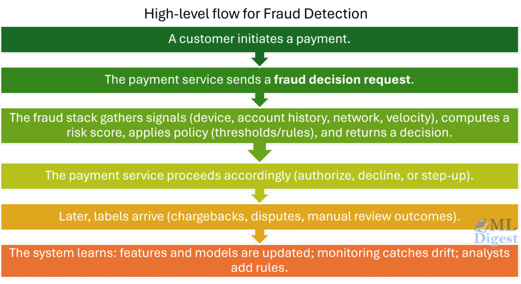
How to Design a Real-Time Fraud Detection System for Payments

Fraud detection for payments is a real-time decision problem under uncertainty:
you must decide to approve, decline, or step-up a payment within milliseconds, while the ground-truth label (chargeback, dispute, confirmed fraud) often arrives hours to weeks later.

Think of it like an airport security line:
most travelers are legitimate and should pass quickly, a small fraction are risky and should be stopped, and some are ambiguous and should be routed for additional checks. The system must keep the line moving while adapting to new threats.

This guide designs a robust, real-time fraud detection system end-to-end: requirements, architecture, online features, modeling and decision policy, evaluation under delayed labels, and production monitoring.

1. High-Level Intuition & Requirements

When a transaction occurs, we have a few milliseconds to decide: Approve, Decline, or Challenge (e.g., ask for 3DS verification). We want to catch as much fraud as possible while minimizing false positives (declining good customers).

The hard part is not producing a score; it is making an action under tight latency, missing labels, and adaptive adversaries.

Before we look at servers and databases, let’s visualize the problem conceptually. A fraud detection system isn’t a single wall; it’s a series of improving filters.

Think of it as three gates:

The Fast Gate (Rules & Allow-lists): “Is this IP on the blacklist? Block them.” This is instant lookup.
The Smart Gate (Machine Learning): “This transaction doesn’t match known fraud patterns. Let’s run it through the model.” This is where the ML model shines, catching subtle patterns.
The Human Gate (Manual Review): “I’m not sure. Let’s pull it aside and ask for a manual review.” This is the slowest but most accurate step for edge cases.

The Problem Space

Designing this is difficult because we fight against three fundamental constraints:

Extreme Imbalance: Genuine transactions vastly outnumber fraud (typically 99.9% vs 0.1%). A model that simply says “Legitimate” to everyone achieves 99.9% accuracy but is useless.
Adversarial Environment: Unlike predicting the weather, your “class 1” (fraudsters) is actively trying to trick your model. If you block IP addresses, they switch to residential proxies. If you block high velocity, they slow down.
Delayed Feedback: You make a prediction at transaction time, but the truth (the label) might arrive at a delay of 30 days (when the bank processes a chargeback). You are constantly training on “old” news to predict the future.

Functional Requirements

Real-time Decisioning: The system must return an Approve/Decline/Review decision within ~50ms of receiving the request.
Explainability: We need to know why a transaction was declined (e.g., “high velocity from new IP”).
Rule & Model Hybrid: Pure ML is too slow to adapt; pure rules are too rigid. We need both.

Non-Functional Requirements

Latency: p99 < 100ms end-to-end.
Scalability: Must handle peaks (e.g., Black Friday) of 50k+ TPS.
Consistency: Features used for training must mathematically match features used for inference.

2. System Architecture

Let’s visualize the flow of data. Imagine the life of a single transaction.

The Two Parallel Worlds

A robust fraud system lives in two worlds simultaneously: the Fast World (Synchronous) and the Slow World (Asynchronous).

1. The Fast World (The Decision Loop – < 100ms)
This is where the fraud decision must be made in real time during the payment authorization flow.

Input: User clicks “Pay”.
Action:
1. Feature Fetch: Grab the user’s history (e.g., “How much did they spend immediately prior to this?”). This requires a specialized Online Feature Store.
2. Model Scoring: Pass features to the ML model (Latency budget: ~20ms).
3. Policy Check: Apply business rules (e.g., “Don’t decline huge revenue partners”).
Output: APPROVE, DECLINE, or CHALLENGE.

2. The Slow World (The Learning Loop – Hours/Days)
This is the the path that the system learns from new data and adapts to emerging fraud patterns.

Chargeback and dispute ingestion: Payment network and issuer feedback.
Analyst Review: Humans review sketchy transactions and label them.
Feedback Ingestion: We receive “Chargeback” files from payment networks (Visa/Mastercard).
Training and validation: model retraining, calibration, offline evaluation.
Deployment: gradual rollout, shadow testing, backtesting.

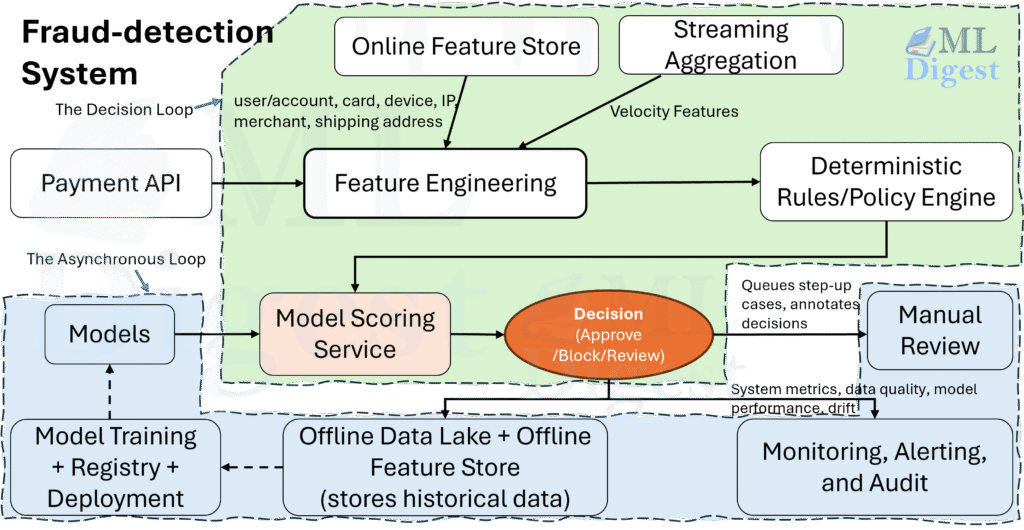
(Fraud Detection Architecture: The decision loop (synchronous path) is fast, streamlined, optimized for speed. The bottom path (asynchronous path) carries massive amounts of history, slower moving, but essential for carrying the “knowledge” back to the starting line.)

Key Components

Risk Orchestrator: The entry point: brain’s coordinator. It creates the “Context” object for the transaction and manages timeouts. If the ML model is too slow, the Orchestrator fails open (approves) or fails closed (declines) based on configuration.
Online Feature Store (e.g., Redis, DynamoDB, Cassandra): The critical component. It bridges the gap. It holds pre-computed aggregations (e.g., “spend_last_1h”).
Feature Computation Engine (e.g., Flink, Kinesis): It watches the stream of events and updates the Online Feature Store in real-time.
Model Serving: Hosts the model artifacts (XGBoost logic, Neural Net weights).
Rule Engine: A fast, in-memory engine to apply business rules along with the model scores.

3. Data & Feature Engineering

Payment API sends:
– transaction context: amount, currency, merchant id, MCC, channel.
– customer context: account id, email hash, phone hash, signups, logins, password resets, profile changes.
– instrument context: card token, BIN, funding type.
– device/network context: device id, IP, proxy/VPN signals, user agent, geo.

While architecture handles the speed, features handle the intelligence. In fraud detection, raw data (like user_id or amount) is rarely enough. The magic lies in velocity and consistency.

We transform raw “facts” into “signals” using three primary techniques:

3.1 Velocity & Windowed Aggregates

Fraudsters are greedy. When they buy a stolen credit card (CVV), they want to drain it before the owner notices. We catch this with Velocity.

Concept: Count events over sliding time windows.
Implementation: We don’t scan the database. We use Streaming Aggregations.
- count(orders) WHERE user_id = X AND time > now() - 10m
- sum(amount) WHERE ip_address = Y AND time > now() - 1h
- count(unique_cards) by device_id over 24h

Why this works: A user spending $500 is normal. A user spending $500 five times in 10 minutes is suspicious.

3.2 Consistency & Profile Matching

Does this transaction match the user’s history?

Geo-Velocity: Calculate the speed required to travel between the last login and the current purchase.
- Example: Login in London at 10:00 AM. Purchase in New York at 11:00 AM. Speed > 3000 mph. -> Fraud.
Device Fingerprinting: “User usually enters from an iPhone 14. Today they are on a Windows 10 desktop with a mismatched screen resolution.”
Merchant category mismatch: “User usually buys electronics, but this transaction is for luxury handbags.”

3.3 Network and Graph Features

Fraudsters often operate in rings. They reuse assets.

Graph Degree: “How many unique credit cards has this generic device attempted to use today?” (High fan-out).
Shared Identity: “Does this email address share a phone number with a known banned account?”

3.4 Reputation & Historical Risk

Some features are based on the reputation of entities:

“Has this card ever been involved in a chargeback?”
“Is this IP address on a known proxy/VPN list?”
“Has this email hash been associated with fraud in the past?”

3.5 Embeddings

Modern systems use Deep Learning to learn representations.
Entity Embeddings map categorical variables (like Merchant ID) to high-dimensional vectors. This allows the model to learn that “Steam Games” and “PlayStation Store” are similar (digital goods, high risk), even if it has never seen a link between them.

3.6 Behavioral Biometrics (Optional)

Some advanced systems also incorporate behavioral biometrics, such as typing patterns, mouse movements, recent password resets, login anomalies or even gait analysis for mobile devices. These can be powerful signals but require careful handling of privacy and latency.

4. Modeling Strategy: The “Swiss Cheese” Defense

No single model is perfect. We need to align multiple models in series to cover each other’s gaps. This is the Layered Defense Strategy.

Layer 1: The Heuristic Rules (The Precision Layer)

Objective: Block obvious bad actors instantly. Cheap to run. Example: IF IP_Country == 'Embargoed' THEN Decline.
Pros: strict compliance, 0ms latency.
Cons: brittle, high maintenance.

Layer 2: The ML Score (The “Brain”)

This is usually a Gradient Boosted Tree (XGBoost, LightGBM) or a Neural Network. It takes hundreds of features and outputs a probability score $[0, 1]$.

Why Gradient Boosting? It handles tabular data, distinct categories, and missing values exceptionally well, which is typical for payment data.

Layer 3: The Policy Layer

We don’t just take the raw score. We apply business logic on top.

“If risk_score > 0.9 BUT user_is_VIP, route to CHALLENGE not DECLINE.”
“If risk_score > 0.8 AND velocity_features indicate a spike, escalate to manual review.”

5. Mathematical Deep Dive: Cost-Sensitive Decisioning

Here is where we switch from engineering to pure mathematics. A model gives you a score $s \in [0, 1]$. The business needs a binary decision $d \in {\text{Approve, Decline}}$.

How do we pick the threshold $\tau$ to map from probability to decision? We minimize Expected Financial Loss.

Let’s define our costs:

Cost of False Negative ($C_{FN}$): We approve fraud.
$$ C_{FN} = \text{Transaction Value} + \text{Chargeback Fee} + \text{Admin Cost} $$
Cost of False Positive ($C_{FP}$): We decline a good user.
$$ C_{FP} = (\text{Transaction Value} \times \text{Margin}) + \text{Lifetime Value Impact (LTV)} $$
Note: The insult of being declined often causes a user to leave forever (Churn).

To decide whether to block a transaction with estimated fraud probability score $s$, we block if the expected cost of fraud exceeds the expected cost of blocking:

$$ s \cdot C_{FN} > (1 – s) \cdot C_{FP} $$

Solving for $s$, we find the optimal threshold $\tau$:

$$ \tau = \frac{C_{FP}}{C_{FN} + C_{FP}} $$

Example:

You lose \$100 on a \$100 fraud (plus fees). Total $C_{FN} \approx \$125$.
You lose \$5 (margin) on a \$100 decline, plus \$20 in future LTV. Total $C_{FP} \approx \$25$.
Threshold $\tau = 25 / (125 + 25) = 25/150 = 1/6 \approx 0.16$

Insight: You should block the transaction if the model thinks there is just a 16% chance of fraud. This counter-intuitive result drives the aggressive nature of fraud systems.

The Calibration Requirement

Crucially, this formula only works if $s$ is a calibrated probability. Most modern ML models (like XGBoost) output raw scores that are not probabilities. They might push all scores towards 0 and 1 (over-confident) or cluster them in the middle.

We Must apply Isotonic Regression (or Platt Scaling) to map raw model scores to calibrated probabilities before applying the threshold formula.

$$ \hat{P}_{\text{calibrated}} = \text{Isotonic}(f(x)) $$

Without calibration, your threshold $\tau$ is just a magic number. With calibration, $\tau$ is derived directly from your business P&L.

6. Evaluation Protocols

Standard metrics like Accuracy are useless. (A model that approves everything has 99.9% accuracy).

6.1 The Censored Data Problem: The “Grey” Area

We never know the true label for transactions we decline.

Did we stop a thief? Maybe.
Did we annoy a VIP? Maybe.
We effectively “blind” ourselves to the results of our own decisions.

The Solution: Control Groups (Exploration)
We randomly set aside 1-5% of traffic as a Control Group.

Exploration Policy: For this group, we disable the blocking rules (or set a very high threshold). We let risky transactions pass.
Result: We buy “labels” with real money. We confirm if high-risk scores actually result in chargebacks. This unbiased data is gold for training the next model version.

6.2 Key Metrics

PR-AUC (Precision-Recall Area Under Curve): The standard for imbalanced classes.
Recall @ Precision X: “What % of fraud do we catch if we enforce that 99% of declines must be valid fraud?”
Chargeback Rate (BPS): Basis Points. The definitive business metric. (e.g., 50 bps implies 0.5% of volume is lost to fraud).
Approval rate and challenge rate: important product metrics that reflect customer friction.

7. Operational Excellence

Building the model is 20% of the work. Keeping it alive is 80%.

7.1 Latency Budgeting (Total: 100ms)

Network Overhead (5ms): The inescapable cost of moving bytes.
Feature Fetch (15ms): This is the biggest bottleneck. Use Redis pipelining or a high-performance store like Aerospike. Parallelism is non-negotiable here.
Model Inference (20ms): Use ONNX or Treelite for faster tree traversal. Consider quantization for neural nets.
Policy & Logic (<5ms): Keep rules simple.

Database Writes (Async): 0ms (Don’t block the response for DB writes!)

7.2 Monitoring the Unknowable

Since true labels (chargebacks) arrive days late, how do you know if your model is broken today?

You monitor the predictions, not the labels.

Prediction Drift: If your model approved 90% of transactions yesterday but only 60% today, you have a problem.
Feature Drift: If the average “Risk Score” of a transaction spikes, check if a specific feature (like “IP Risk”) has changed.
Operational Metrics: Is Redis latency spiking? Are timeouts increasing?

7.3 The “Kill Switch”

Models drift. Attacks change. If your Neural Net starts declining 50% of traffic on Black Friday, what do you do?

Safe Mode: A physical config switch that bypasses the ML Model and falls back to a whitelist/blacklist Rules engine.
Shadow Mode: Always run the next version of the model in “shadow mode” (scoring but not deciding) for weeks before promoting it to “live”.

8. Summary

Designing a fraud system is a practice in balancing opposing forces:

Speed vs. Complexity
False Positives (Insult) vs. False Negatives (Loss)
Exploration (Learning) vs. Exploitation (Blocking)

The best systems are not just “big models”; they are fast feedback loops that turn yesterday’s attack into today’s training data.

Subscribe to our newsletter!