Imagine that you need to open $K$ new coffee shops in a city. You want each person to walk to the nearest shop, and you want the total walking distance across the city to be as small as possible.
You could start by dropping $K$ candidate locations on the map. Once the locations are fixed, every resident naturally chooses the closest shop. That creates $K$ neighborhoods. Then you ask a second question: if a shop must serve the people currently assigned to it, where should it move? The best answer is the center of that neighborhood. After the shops move, some residents switch to a different shop, which creates new neighborhoods. Repeating these two actions eventually stabilizes the system.
That alternating rhythm is the heart of K-means clustering:
- Assign each point to the nearest center.
- Move each center to the mean of its assigned points.
K-means is one of the most widely used unsupervised learning algorithms because it turns a vague idea, “group nearby things together,” into a simple and efficient optimization procedure. In this article, we will build that intuition first, then connect it to the objective function, convergence behavior, and practical usage.
1. The Intuition: Grouping Around Prototypes
At a high level, K-means is a prototype-based clustering algorithm. Each cluster is represented by a prototype, called a centroid, and every data point belongs to the cluster with the nearest centroid.
The difficulty is that clustering has a circular structure:
- If we knew the centroids, assigning points to clusters would be easy.
- If we knew the cluster assignments, computing the best centroids would also be easy.
We start with neither. K-means resolves this by alternating between the two easy subproblems until the assignments stop changing.
1.1 What K-means is Really Learning
It helps to be precise about what the algorithm is and is not learning.
- It is not learning arbitrary cluster shapes.
- It is learning a set of $K$ representative locations in feature space.
- It uses those locations to partition the space into regions where each region contains all points closest to one centroid.
In other words, K-means does not search for a complex boundary first. It searches for good representatives, and the boundaries emerge as a consequence.
1.2 The Illustrated Iteration
Let us visualize the process on a 2D plane.
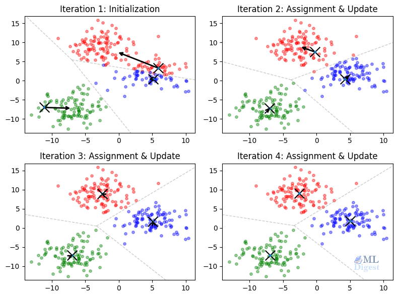
- Initialization: We place $K$ centroids on the plot, often by random selection or with the smarter
k-means++strategy. - Assignment step: Each point is assigned to the nearest centroid. Geometrically, this forms a Voronoi partition of the plane, where every region contains the locations closer to one centroid than to any other.
- Update step: For each cluster, we compute the arithmetic mean of the assigned points and move the centroid there.
- Repeat: Because the centroids moved, the Voronoi regions change, some points switch clusters, and the process repeats.
This procedure is commonly called Lloyd’s algorithm. It is simple, but it hides an important fact: every iteration is trying to reduce a well-defined objective.
2. Why K-means Matters
Despite its age, K-means remains a core algorithm in machine learning because it occupies an important sweet spot: it is conceptually simple, computationally efficient, and often strong enough for a first practical baseline.
- Fast on large datasets: The algorithm is highly efficient. Its time complexity is approximately $O(n \cdot K \cdot I \cdot d)$, where $n$ is the number of points, $K$ is the number of clusters, $I$ is the number of iterations, and $d$ is the number of dimensions. Since $K$, $I$, and $d$ are generally much smaller than $n$, the algorithm scales linearly with the size of the dataset. This makes it substantially cheaper than models like hierarchical clustering, which scales at $O(n^3)$.
- Easy to interpret: Each cluster is summarized by a centroid, which gives a concrete representative of the group.
- Useful as a building block: K-means appears inside vector quantization, codebook learning, bag-of-visual-words pipelines, image compression, and even some initialization procedures for more advanced models.
Common Use Cases
- Customer segmentation: Group customers by behavior, spending patterns, or engagement signals.
- Image compression: Replace many pixel colors with a smaller learned palette of centroid colors.
- Document clustering: Group vectorized documents into coarse topics.
- Anomaly detection: Flag points that are unusually far from their nearest centroid.
K-means is often the right first question to ask of a dataset: “If I force this data into $K$ groups around $K$ prototypes, does the result reveal useful structure?”
3. The Mathematical Rigor
Now we can formalize the story. K-means solves an optimization problem: find cluster assignments and centroids that minimize the total squared distance between each point and the centroid of the cluster it belongs to.
3.1 Objective Function (Inertia)
The K-means objective, often called inertia or within-cluster sum of squares (WCSS), is
$$
J = \sum_{i=1}^{n} \sum_{k=1}^{K} r_{ik} \lVert x^{(i)} – \mu_k \rVert_2^2
$$
where:
- $n$ is the number of data points,
- $K$ is the number of clusters,
- $x^{(i)}$ is the $i$-th data point,
- $\mu_k$ is the centroid of cluster $k$,
- $r_{ik}$ is a binary assignment indicator with value $1$ if point $i$ is assigned to cluster $k$, and $0$ otherwise.
Only one $r_{ik}$ can be $1$ for a given point, so each point contributes exactly one squared distance term to the objective.
This objective reveals an important geometric bias: K-means prefers clusters whose points stay close to a single central location under squared Euclidean distance. That is why it works best for compact, roughly spherical clusters.
3.2 Why the Assignment Step is Optimal
Suppose the centroids $\mu_1, \dots, \mu_K$ are fixed. Then the only remaining decision is: which cluster should each point join?
For a single point $x^{(i)}$, the objective contributes
$$
\sum_{k=1}^{K} r_{ik} \lVert x^{(i)} – \mu_k \rVert_2^2
$$
Since exactly one assignment variable equals $1$, minimizing this term means choosing the centroid with the smallest squared distance. Therefore,
$$
r_{ik} = \begin{cases}
1 & \text{if } k = \arg\min_j \lVert x^{(i)} – \mu_j \rVert_2^2 \
0 & \text{otherwise}
\end{cases}
$$
So the assignment step is not just intuitive. It is the exact minimizer of $J$ when the centroids are held fixed.
3.3 Why the Update Step Produces the Mean
Now suppose the assignments are fixed. Then we minimize $J$ with respect to each centroid $\mu_k$ independently.
For cluster $k$, we solve
$$
\min_{\mu_k} \sum_{i=1}^{n} r_{ik} \lVert x^{(i)} – \mu_k \rVert_2^2
$$
Taking the derivative with respect to $\mu_k$ and setting it to zero gives
$$
\frac{\partial J}{\partial \mu_k} = \sum_{i=1}^{n} r_{ik} 2(\mu_k – x^{(i)}) = 0
$$
Rearranging,
$$
\mu_k \sum_{i=1}^{n} r_{ik} = \sum_{i=1}^{n} r_{ik} x^{(i)}
$$
and therefore
$$
\mu_k = \frac{\sum_{i=1}^{n} r_{ik} x^{(i)}}{\sum_{i=1}^{n} r_{ik}}
$$
This is exactly the arithmetic mean of the points assigned to cluster $k$. The name K-means comes directly from this update rule.
3.4 Convergence: Coordination and Expectation-Maximization
The full algorithm is an elegant form of coordinate descent. We alternate between two distinct optimization paths:
- Hold centroids fixed, optimize assignments: This is functionally identical to the “Expectation” step in the Expectation-Maximization (EM) algorithm. We estimate the latent variables, deciding exactly which point belongs to which cluster.
- Hold assignments fixed, optimize centroids: This represents the “Maximization” step. We update our model parameters (the centroids) to maximize the likelihood of the data given our recent assignments.
Unlike Gaussian Mixture Models that assign a “soft” probability of belonging to various clusters, K-means creates “hard” assignments, meaning a point is either completely in cluster $A$ or completely in cluster $B$. Each alternating step decreases the objective $J$ or leaves it unchanged. Because there are only finitely many ways to assign $n$ points to $K$ clusters, the process mathematically must eventually stop changing. Once it ceases to change, the algorithm has successfully converged.
3.5 Convergence Does Not Mean Global Optimality
This convergence guarantee is useful, but it is limited. K-means is guaranteed to reach a local minimum, not the global optimum. Different initial centroid placements can lead to different final solutions.
That is why initialization matters so much. A poor starting configuration can trap the algorithm in a suboptimal partition, as illustrated below.

This is also why implementations usually run K-means multiple times with different seeds and keep the best result.
4. Practical Implementation with Python
We will now implement K-means using scikit-learn for a production-ready workflow. The code is straightforward, but the modeling choices around it matter far more than the few lines needed to fit the model.
4.1 Preprocessing is Not Optional
K-means is entirely driven by distances. That means the numerical scale of the input features directly controls the geometry of the clusters.
If one feature such as salary ranges in the thousands, while another such as age ranges in the tens, salary will dominate the Euclidean distance calculation. In practice, the algorithm will behave as if age barely exists.
That is why feature scaling is usually mandatory. Standardization with StandardScaler is a common default because it puts features on comparable scales.
There is a second practical implication here: K-means expects a meaningful Euclidean geometry. Raw categorical features, arbitrary IDs, and poorly engineered sparse features can make that geometry misleading. When K-means fails in practice, the issue is often the representation, not the optimizer.
4.2 Production Code Example
Here is a complete, runnable workflow using scikit-learn. We use k-means++ initialization, which spreads the initial centroids more intelligently than naive random selection and usually leads to faster and more stable convergence.
import numpy as np
import matplotlib.pyplot as plt
from sklearn.cluster import KMeans
from sklearn.preprocessing import StandardScaler
from sklearn.datasets import make_blobs

# 1. Generate synthetic data
# We create 300 samples with 4 distinct centers (blobs)
X, y_true = make_blobs(n_samples=300, centers=4, cluster_std=0.60, random_state=0)

# 2. Preprocessing
# Standardize features by removing the mean and scaling to unit variance
scaler = StandardScaler()
X_scaled = scaler.fit_transform(X)

# 3. Fit K-Means
# Setting n_init explicitly to 10 ensures we run multiple initializations
# and keep the best one, avoiding poor local minima.
kmeans = KMeans(
    n_clusters=4,
    init='k-means++',
    n_init=10,
    random_state=42
)
kmeans.fit(X_scaled)

# 4. Results
y_kmeans = kmeans.predict(X_scaled)
centers = kmeans.cluster_centers_

# 5. Visualization (since we are in 2D)
plt.figure(figsize=(8, 6))
plt.scatter(X_scaled[:, 0], X_scaled[:, 1], c=y_kmeans, s=50, cmap='viridis', marker='o', edgecolor='k', label='Data Points')
plt.scatter(centers[:, 0], centers[:, 1], c='red', s=200, alpha=0.75, marker='X', label='Centroids')
plt.title('K-means Clustering Results')
plt.xlabel('Feature 1 (standardized)')
plt.ylabel('Feature 2 (standardized)')
plt.legend()
plt.grid(True)
plt.show()

# 6. Inverse transform centroids to interpret them in original units
original_centers = scaler.inverse_transform(centers)
print("Cluster Centers (Original Units):")
print(original_centers)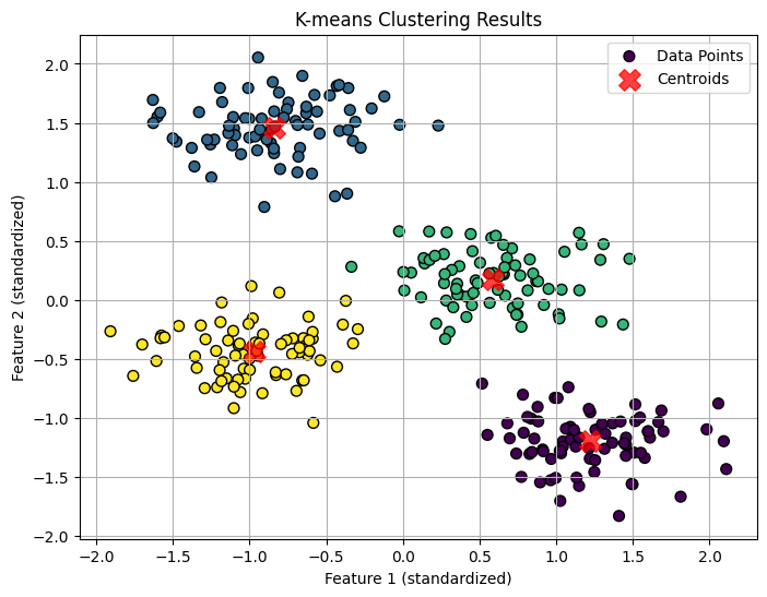
4.3 Key Parameters Explained
n_clusters($K$): The number of clusters to find. This is the most important hyperparameter because the algorithm does not infer it automatically.init='k-means++': Instead of placing centroids arbitrarily, this method tends to seed them far apart, which reduces the chance of poor local minima.n_init: The number of independent restarts with different initial centroid placements. The final result is the run with the lowest inertia.
5. Choosing the Right $K$
Choosing $K$ is often harder than running the algorithm itself. K-means will always return exactly $K$ clusters, even if the data does not naturally contain that many groups, so this choice should be made deliberately.
Two common heuristics help guide the decision.
5.1 The Elbow Method
We run K-means for a range of $K$ values, such as $1$ through $10$, and plot the inertia for each value. Since adding more clusters always gives the model more flexibility, inertia will keep decreasing as $K$ grows.
The key question is not whether inertia decreases, because it always does. The question is whether the decrease is still meaningful. The so-called elbow is the point where adding another cluster produces only a modest improvement.
Click to check the code.
import numpy as np
import matplotlib.pyplot as plt
from sklearn.cluster import KMeans
from sklearn.datasets import make_blobs

# 1. Generate synthetic data with 5 natural clusters
X, _ = make_blobs(n_samples=500, centers=5, cluster_std=0.7, random_state=42)

# 2. Calculate inertia for a range of K values
inertias = []
k_range = range(1, 11)

for k in k_range:
    model = KMeans(n_clusters=k, n_init=10, random_state=42)
    model.fit(X)
    inertias.append(model.inertia_)

# 3. Plot the Elbow Method curve
fig, ax = plt.subplots(figsize=(6, 4))
ax.plot(k_range, inertias, 'bo-')
ax.set_xlabel('Number of Clusters (K)')
ax.set_ylabel('Inertia (Within-cluster Sum of Squares)')
ax.set_title('The Elbow Method showing the optimal K')
ax.set_xticks(list(k_range))
ax.grid(True)

# Annotate the elbow point
ax.annotate('Elbow Point', xy=(5, inertias[4]), xytext=(6, inertias[4] + 2500),
             arrowprops=dict(facecolor='black', shrink=0.05))

plt.show()
This is a useful heuristic, but it is not a theorem. Some datasets show a clear elbow, while many real datasets do not.
5.2 The Silhouette Score
The silhouette score measures how well a point fits inside its assigned cluster compared with the next-best alternative cluster. It balances two ideas:
- Cohesion: points should be close to others in the same cluster.
- Separation: points should be far from points in neighboring clusters.
The score ranges from $-1$ to $1$:
- Near $1$: clusters are well separated.
- Near $0$: clusters overlap.
- Below $0$: many points may be assigned to the wrong cluster.
In practice, we compute the average silhouette score across points for several values of $K$ and prefer the one with the highest score.
Click to check the code.
import numpy as np
import matplotlib.pyplot as plt
from sklearn.cluster import KMeans
from sklearn.metrics import silhouette_score
from sklearn.datasets import make_blobs

# 1. Generate synthetic data with 5 natural clusters
X, _ = make_blobs(n_samples=500, centers=5, cluster_std=0.7, random_state=42)

# 2. Calculate Silhouette Scores for a range of K values
silhouette_avg = []
k_range = range(2, 11) # Silhouette score requires at least 2 clusters

for k in k_range:
    kmeans = KMeans(n_clusters=k, n_init=10, random_state=42)
    cluster_labels = kmeans.fit_predict(X)

    # The silhouette_score gives the average value for all the samples.
    silhouette_avg.append(silhouette_score(X, cluster_labels))

# 3. Plotting the Silhouette Scores
fig, ax = plt.subplots(figsize=(6, 4))
ax.plot(k_range, silhouette_avg, 'ro-')
ax.set_xlabel('Number of Clusters (K)')
ax.set_ylabel('Average Silhouette Score')
ax.set_title('Silhouette Analysis for Optimal K')
ax.set_xticks(list(k_range))
ax.grid(True)

# Find the K with the maximum score
optimal_k = k_range[np.argmax(silhouette_avg)]
ax.annotate(f'Optimal K={optimal_k}', xy=(optimal_k, max(silhouette_avg)),
             xytext=(optimal_k, max(silhouette_avg) - 0.15),
             arrowprops=dict(facecolor='black', shrink=0.05))

plt.show()
However, silhouette analysis still inherits K-means’ geometric preferences. It is most informative when clusters are compact and well separated under Euclidean distance.
6. Implementation from Scratch (Educational)
To make Lloyd’s algorithm feel less mysterious, it is helpful to implement a minimal version with numpy. This version is excellent for intuition and debugging, even though a production library implementation will be more optimized and robust.
import numpy as np
import matplotlib.pyplot as plt

def simple_kmeans(X, n_clusters, max_iters=100, tolerance=1e-4, seed=42):
    rng = np.random.default_rng(seed)

    # --- Step 1: Initialization ---
    initial_indices = rng.choice(X.shape[0], n_clusters, replace=False)
    initial_centroids = X[initial_indices]
    centroids = initial_centroids.copy()

    # Capture initial labels for the first plot
    initial_distances = np.linalg.norm(X[:, np.newaxis] - initial_centroids, axis=2)
    initial_labels = np.argmin(initial_distances, axis=1)

    for i in range(max_iters):
        # --- Step 2: Assignment ---
        distances = np.linalg.norm(X[:, np.newaxis] - centroids, axis=2)
        labels = np.argmin(distances, axis=1)

        # --- Step 3: Update ---
        new_centroids = np.array([X[labels == k].mean(axis=0) if np.any(labels == k) else centroids[k] for k in range(n_clusters)])

        # --- Step 4: Check Convergence ---
        if np.linalg.norm(new_centroids - centroids) < tolerance:
            print(f"Converged at iteration {i}")
            break
        centroids = new_centroids

    return initial_centroids, initial_labels, centroids, labels

# Run the manual implementation
init_centers, init_labels, final_centers, final_labels = simple_kmeans(X_scaled, n_clusters=4)

# Visualization
fig, (ax1, ax2) = plt.subplots(1, 2, figsize=(10, 4))

# Plot 1: Initialization
ax1.scatter(X_scaled[:, 0], X_scaled[:, 1], c=init_labels, cmap='viridis', s=20, alpha=0.5)
ax1.scatter(init_centers[:, 0], init_centers[:, 1], c='red', marker='X', s=100, label='Initial Centroids')
ax1.set_title("Initial State (Random Selection)")
ax1.legend()

# Plot 2: Final Result
ax2.scatter(X_scaled[:, 0], X_scaled[:, 1], c=final_labels, cmap='viridis', s=20, alpha=0.5)
ax2.scatter(final_centers[:, 0], final_centers[:, 1], c='red', marker='X', s=100, label='Final Centroids')
ax2.set_title("Final State (Converged)")
ax2.legend()

plt.show()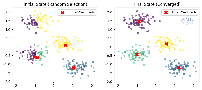
7. When K-means Works Well, and When It Fails
K-means is powerful precisely because it is simple. But that simplicity comes with assumptions. It is best used when those assumptions roughly match the geometry of the data.
7.1 Best-Case Scenario for K-means
K-means tends to work well when:
- clusters are compact;
- clusters are reasonably separated;
- cluster variance is roughly equal across groups (K-means assumes spherical clusters of the same radius);
- Euclidean distance is a meaningful similarity measure.
In these settings, the centroid is a sensible summary of a cluster, and minimizing squared distance aligns well with our intuitive notion of grouping. Under the hood, K-means is mathematically equivalent to a Gaussian Mixture Model where we strictly assume all clusters are spherical and share the exact same variance.
7.2 Non-Spherical and Unequal-Variance Clusters
K-means struggles significantly when the true clusters are elongated, curved, nested, or ring-shaped. A crescent-shaped dataset is the classic failure case: because K-means relies solely on Euclidean distance from a central point, it will rigidly cut the crescents into centroid-friendly, spherical chunks rather than discovering the true curved structure.
Furthermore, if one cluster is naturally very dense and compact while another is sparse and wide, K-means will often misassign points from the wide cluster to the dense one. The algorithm does not possess the capacity to adapt its boundary radius on a per-cluster basis; it enforces rigid, equidistant Voronoi boundaries.
This happens because the model is not searching for arbitrary cluster boundaries. It is searching for partitions induced by nearest-centroid regions.
For non-linear cluster shapes, methods such as DBSCAN, Spectral Clustering, or hierarchical approaches are often better suited.
7.3 Sensitivity to Outliers
Because the objective squares distances, a single extreme point can pull a centroid disproportionately far from the dense core of the cluster.
That makes K-means much more sensitive to outliers than its simple interface suggests. In practice, it is often worth:
- removing obvious outliers,
- clipping extreme values,
- or considering alternatives such as K-medoids when robustness matters.

7.4 High-Dimensional Data
In high-dimensional spaces, pairwise Euclidean distances often become less informative. Points can start to look similarly far from one another, which weakens the geometric signal K-means relies on.
That is one reason why text clustering with raw high-dimensional sparse vectors can be tricky. In such cases, dimensionality reduction, better embeddings, or cosine-based variants such as spherical K-means may be more appropriate.
7.5 Empty Clusters and Practical Edge Cases
One subtle implementation detail is that a cluster can become empty during an iteration if no points are assigned to its centroid. Robust implementations handle this explicitly, often by reinitializing that centroid.
This edge case is another reminder that K-means is easy to describe but still requires careful engineering in practice.
Summary
K-means remains one of the most useful entry points into unsupervised learning because its mechanics are so transparent. It alternates between two exact subproblems, assigning points to the nearest centroid and updating each centroid to the mean of its assigned points, and in doing so it steadily reduces a clear objective.
Its strengths are speed, simplicity, and interpretability. Its weaknesses come from the same place: it assumes that clusters can be represented well by means under squared Euclidean distance.
If you remember only the practical lessons, remember these three:
- Scale your features.
- Use multiple initializations, preferably with
k-means++. - Treat the choice of $K$ as a modeling decision, not a default.
When those conditions are respected, K-means is often an excellent baseline and, quite often, a strong final solution.

Happy is a seasoned ML professional with over 15 years of experience. His expertise spans various domains, including Computer Vision, Natural Language Processing (NLP), and Time Series analysis. He holds a PhD in Machine Learning from IIT Kharagpur and has furthered his research with postdoctoral experience at INRIA-Sophia Antipolis, France. Happy has a proven track record of delivering impactful ML solutions to clients.
Subscribe to our newsletter!