Decision trees are one of the simplest ways to turn data into a sequence of human-readable rules. You can think of a decision tree as a careful game of “20 Questions”: at each step, the model asks a yes/no question about a feature, and each question is chosen to make the remaining uncertainty about the target as small as possible. After a few questions, you arrive at a leaf node that outputs a prediction.
If you want a concrete mental picture, imagine a triage flowchart on a whiteboard:
- “Is temperature above 38°C?”
- “Is cough present?”
- “Did symptoms start within 48 hours?”
Each question narrows the case to a smaller and more internally consistent group. A decision tree does the same thing, except the questions, thresholds, and ordering are learned from data rather than written manually.
That combination makes decision trees unusually valuable in practice. They are easy to explain, often strong enough to serve as a serious baseline, and conceptually rich enough to teach core ideas such as impurity, recursive partitioning, overfitting, and regularization. They also sit at the center of modern tabular machine learning because many strong ensemble methods, such as random forests and gradient boosting, are built from trees.
This article focuses on the single decision tree as a model in its own right. The goal is to build a layered understanding: first the intuition, then the mathematics of splitting, then the practical issues that determine whether a tree generalizes well or simply memorizes the training set.
1. What Makes a Decision Tree Different from Hand-Written Rules
A decision tree is a data-driven rule learner. It searches over many possible questions and keeps the ones that most reduce uncertainty about the target.
That is the crucial difference from a manually designed rule system:
- Hand-written rules come from intuition, domain expertise, or policy.
- Decision trees infer rules from examples.
- Hand-written rules are often static.
- Decision trees adapt when the data distribution changes and the model is retrained.
This distinction matters because a tree can uncover interactions a human might not think to encode explicitly. For example, a domain expert might check age and income separately, while a tree may discover that income matters differently for younger and older customers because the split sequence naturally models interactions.
At the same time, a decision tree is not “intelligent” in a broad sense. It does not reason symbolically about the world. It only optimizes a training objective over the observed data. If the data are biased, noisy, or leaky, the learned rules will reflect those problems.
2. Why Decision Trees Matter
Decision trees matter because they occupy a useful middle ground in the model landscape. Linear models are simple and often robust, but they can struggle when the signal depends on interactions or threshold effects. Highly flexible nonlinear models can capture those patterns, but they are often harder to inspect and communicate. A single decision tree offers a compromise: more expressive than a linear boundary, yet still readable as a sequence of decisions.
Another reason they matter is pedagogical. Many ideas that appear later in more advanced models already show up here in simplified form: greedy optimization, bias-variance trade-offs, regularization, calibration issues, and the danger of leakage. If you understand a tree deeply, many ensemble methods become easier to understand as well.
2.1 Strengths
- Interpretability: A trained tree can be read as rules like “if
age < 35andincome > 80k, then …”. - Nonlinear decision boundaries: Trees can model interactions and piecewise-constant functions.
- Minimal feature engineering: Trees are often competitive without heavy transformations.
- Mixed feature types: With appropriate preprocessing, trees handle numeric and categorical features well.
2.2 Limitations
- Overfitting is easy: An unrestricted tree can memorize noise.
- Instability: Small data changes can lead to a very different tree.
- Axis-aligned splits: Standard trees split on one feature at a time, producing “rectangular” regions.
- Bias toward high-cardinality features: Certain split criteria can prefer features with many unique values.
2.3 Where Trees Commonly Shine
- Tabular business data (credit risk, churn, fraud features, operational forecasting features).
- Problems where stakeholders need explanations.
- As base learners for ensembles (random forests, gradient boosting), which often dominate on tabular benchmarks.
2.4 When a Single Tree Is Usually the Wrong Tool
It is just as useful to know when not to reach for a single tree.
- When the signal is smooth and additive, a linear or generalized linear model may be more stable.
- When the decision boundary is highly oblique or curved, a single axis-aligned tree may need many splits to approximate it well.
- When you care more about predictive performance than direct interpretability, ensembles of trees usually outperform a single tree by a wide margin.
That last point is worth emphasizing: the single tree is often the best teaching model and a strong baseline model, but not always the best final model.
3. How a Decision Tree Makes Predictions
A decision tree partitions feature space into regions and assigns one prediction to each region. In most modern implementations (including CART and scikit-learn), the tree is a binary tree: each internal node tests a condition and sends examples either left or right.
You can think of prediction as a two-stage process:
- Route the example through a sequence of splits.
- Read out the prediction stored in the leaf that the example reaches.
Training decides the routing rules. Inference simply follows them.
3.1 Visual Representation of the Tree and Decision Boundaries
Imagine a 2D dataset with features $x_1$ and $x_2$.
- A split like “$x_1 \le t$” draws a vertical line at $t$.
- A split like “$x_2 \le t$” draws a horizontal line at $t$.
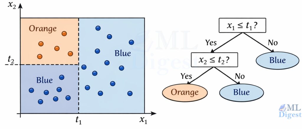
After several splits, the plane becomes a grid of rectangles. Each rectangle corresponds to a leaf node. That geometric picture is important because it explains both the power and the limitations of the model: trees are excellent at carving space into simple local regions, but they do so with axis-aligned cuts.
If you were to draw the tree itself, it would look like a flowchart:
- Root: all examples
- Internal nodes: one question (split)
- Edges: the split outcomes
- Leaves: predicted class (classification) or predicted value (regression)
A key intuition for decision trees is that they partition the feature space into hyper-rectangles. Because every split is of the form $x_i \le t$, the decision boundaries are always orthogonal to the feature axes.
- In 1D (one feature), the tree splits the line into segments.
- In 2D (two features), the tree splits the plane into boxes. (nice visual here)
- In 3D (three features), the tree splits the volume into cuboids.
Why this matters:
This axis-aligned property means standard trees struggle to capture diagonal or rotated relationships compactly. If the true boundary is $x_1 = x_2$ (a diagonal line), a tree usually approximates it with a staircase pattern of many vertical and horizontal cuts. In some problems, rotating the representation first, for example with PCA or learned feature transformations, can make the structure easier for the tree to express.
3.2 Classification vs Regression Trees
- Classification tree: leaves output a class label (or class probabilities).
- Regression tree: leaves output a numeric value, typically the mean of the targets in that leaf.
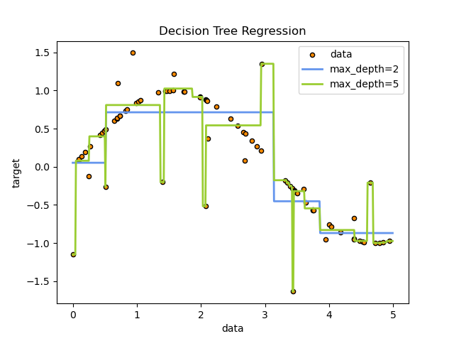
One subtle but important implication is that regression trees are piecewise constant. Inside each leaf, every point receives the same prediction. This is why single regression trees tend to produce blocky prediction surfaces and why they do not extrapolate smoothly beyond the patterns seen in training.
3.3 What the Tree Stores (What Gets Learned)
It helps to demystify what “training” produces. A fitted decision tree is essentially a set of parameters:
- For each internal node: a feature index, a threshold (or category test), and pointers to left and right children.
- For each leaf: a prediction.
In classification, the leaf prediction is often derived from class counts. Many libraries store the vector of class frequencies at each leaf, which allows:
predictto return the argmax class.predict_probato return estimated class probabilities.
These probabilities are often useful, but they should not automatically be interpreted as well-calibrated probabilities. A leaf that contains 9 positives and 1 negative may produce a score of $0.9$, but that does not guarantee the model is well calibrated in the probabilistic sense.
In regression, the leaf typically stores the mean target value (and sometimes additional statistics used for split scoring).
3.4 A Crucial Limitation: Greedy Training
Decision tree training is usually greedy. At each node, the algorithm chooses the split that looks best right now according to the local impurity reduction. It does not search over all possible future trees and therefore does not guarantee a globally optimal tree.
This point is easy to underestimate. In principle, the best overall tree is a combinatorial object: changing the root split changes which candidate splits are available deeper in the tree, which then changes the entire downstream structure. Exhaustively searching that space is computationally infeasible except for tiny problems, so practical algorithms settle for a sequence of locally good decisions.
This is one of the most important conceptual points in the whole article:
- The learned tree can be very good.
- The learned tree is rarely the unique best tree.
- Small changes in data can change early splits, which can change the entire downstream structure.
This explains both the strength and the instability of decision trees. They are flexible and efficient, but the greedy construction process makes them sensitive to local decisions. In practice, this is one reason pruning, minimum leaf sizes, and ensembles help so much: they compensate for the variance introduced by greedy fitting.
4. The Mathematics of Splitting: “Best Question Next”
The core training loop is simple:
- Consider many candidate splits.
- Score each split by how much it improves purity (classification) or reduces error (regression).
- Choose the split with the best score.
- Recurse on child nodes until a stopping criterion triggers.
To define “best,” we need an objective. In classification, “best” usually means producing child nodes that are more class-pure than the parent. In regression, it means producing child nodes whose target values are less dispersed.
4.1 Notation
Let a node contain a dataset $S$ with $n = |S|$ examples.
- For classification with $K$ classes, let $p_k$ be the fraction of examples in class $k$ at that node.
- A candidate split partitions $S$ into children $S_1, S_2, \dots, S_m$.
For binary trees, which are the standard case in CART, $m=2$.
4.2 Impurity Measures for Classification
Entropy
Entropy measures uncertainty:
$$
H(S) = -\sum_{k=1}^{K} p_k \log_2(p_k)
$$
Properties:
- $H(S) = 0$ when the node is pure (all examples in one class).
- Entropy is maximized when classes are uniformly mixed.
An intuitive way to read entropy is: how surprised would I be by the class label if I sampled an example from this node? Pure nodes are unsurprising. Mixed nodes are uncertain.
Information Gain
Information gain measures how much uncertainty is reduced by splitting:
$$
IG(S, \text{split}) = H(S) – \sum_{i=1}^{m} \frac{|S_i|}{|S|} H(S_i)
$$
The algorithm chooses the split with the highest $IG$.
So the tree is not trying to make children small. It is trying to make children informative. A good split creates branches that are easier to predict than the parent node was.
The weighted average in the formula is essential. A split should not look good simply because it creates one tiny pure child and one large messy child. The children are weighted by how many examples they contain, so large branches matter proportionally more.
A Worked Example: One Split, Numbers Included
Consider a binary classification node with $n=10$ examples: 6 positives and 4 negatives.
- Parent class probabilities: $p_+=0.6$, $p_-=0.4$
The parent entropy is:
$$
H(\text{parent}) = -0.6\log_2(0.6) – 0.4\log_2(0.4) \approx 0.971
$$
Now consider a candidate threshold split that produces:
- Left child: 5 examples (4 positives, 1 negative)
- Right child: 5 examples (2 positives, 3 negatives)
The child entropies are:
$$
H(\text{left}) = -0.8\log_2(0.8) – 0.2\log_2(0.2) \approx 0.722
$$
$$
H(\text{right}) = -0.4\log_2(0.4) – 0.6\log_2(0.6) \approx 0.971
$$
The weighted child entropy is:
$$
\frac{5}{10}H(\text{left}) + \frac{5}{10}H(\text{right}) = 0.5\cdot 0.722 + 0.5\cdot 0.971 = 0.8465
$$
So the information gain is:
$$
IG = 0.971 – 0.8465 = 0.1245
$$
This is the entire training decision at a node: evaluate many candidate splits like this, pick the one with the highest impurity reduction, and repeat recursively.
Gini Impurity (CART default)
Gini impurity is another common impurity measure:
$$
G(S) = 1 – \sum_{k=1}^{K} p_k^2
$$
Gini is often slightly faster to compute and behaves similarly to entropy in practice.
An intuitive reading of Gini is: if I randomly label an example according to the class proportions in this node, how often would I be wrong? Lower Gini means the node is easier to classify correctly.
One practical note: information gain can prefer high-cardinality categorical features when categories are not handled carefully. This is one reason many pipelines use one-hot encoding, target-aware ordering methods in specialized libraries, or alternative criteria such as gain ratio in algorithms like C4.5.
In practice, entropy and Gini usually rank candidate splits similarly. The important idea is not which one is philosophically superior, but that both reward splits that make the child nodes more homogeneous than the parent.
4.3 Split Objectives for Regression
In regression, “purity” is replaced by “low variance.” A common objective is to minimize the sum of squared errors (SSE). The model asks: after the split, are the target values inside each child more tightly clustered around a simple constant prediction?
At a node with targets ${y_j}_{j=1}^{n}$, the leaf prediction is often:
$$
\hat{y} = \frac{1}{n}\sum_{j=1}^{n} y_j
$$
For a candidate split into children $S_i$, the score can be the reduction in SSE:
$$
\Delta \mathrm{SSE} = \mathrm{SSE}(S) – \sum_{i=1}^{m} \mathrm{SSE}(S_i)
$$
where
$$
\mathrm{SSE}(S) = \sum_{j \in S} (y_j – \bar{y}_S)^2
$$
This criterion is tightly connected to the fact that the mean minimizes squared error. That is why the average target in a leaf is the natural regression prediction under squared loss.
This also explains the characteristic shape of a regression tree’s prediction function. Since each leaf predicts a single constant, the model approximates a continuous relationship with a step function. That can work surprisingly well on tabular data, but it also means single trees are poor extrapolators.
4.4 How Candidate Splits Are Generated
4.4.1 Numeric Features
For a numeric feature $x$, a common approach is:
- Sort the unique values of $x$ in the node.
- Consider thresholds between consecutive unique values, typically midpoints.
- Evaluate impurity reduction for each threshold.
This is why decision tree training can be computationally heavy on wide datasets, and why optimized implementations use careful sorting and bookkeeping.
Computational intuition: at a node with $n$ examples and $d$ numeric features, evaluating splits naively is expensive. A common optimized pattern is “sort once per feature, then scan thresholds,” which is closer to $O(d\,n\log n)$ per node for sorting plus $O(d\,n)$ scanning, with many additional optimizations in production libraries.
4.4.2 Categorical Features
There are several strategies:
- One-hot encode categories and split on the binary columns.
- Ordered grouping for small cardinality (try subsets), which can be expensive.
- Target-based ordering for binary classification (order categories by positive rate), then treat as numeric; this is used in some implementations.
In practice, in scikit-learn, the most robust default is to use OneHotEncoder for categorical features before fitting a standard tree.
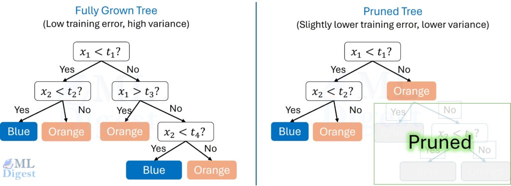
5. Stopping Criteria, Regularization, and Pruning
If you keep splitting until every leaf is perfectly pure (or nearly pure), the tree often overfits. Regularization controls tree complexity.
Another way to say it is that decision trees have low bias and high variance: they can fit very complex patterns, but they can also chase noise unless you constrain them.
There are two broad pruning families of control:
- Pre-pruning: stop growth early.
- Post-pruning: grow a large tree first, then cut back the branches that do not justify their complexity.
Both aim at the same trade-off: allow enough structure to capture real signal, but not so much that the tree starts encoding accidents of the training set.
5.1 Common Pre-Pruning Controls
These stop growth early:
max_depth: maximum depth of the tree.min_samples_split: minimum samples required to split an internal node.min_samples_leaf: minimum samples required at a leaf node.max_leaf_nodes: maximum number of leaves.min_impurity_decrease: require a minimum improvement to split.
Practical intuition:
min_samples_leafis often a strong, stable regularizer because it prevents tiny, noisy pockets from becoming separate leaves.max_depthis useful as a simple cap, but it can be too blunt because all branches are forced to stop at the same depth regardless of local complexity.
5.2 Post-Pruning (Cost-Complexity Pruning)
Cost-complexity pruning shrinks a fully grown tree by penalizing the number of leaves.
One common formulation:
$$
R_\alpha(T) = R(T) + \alpha \cdot |\text{leaves}(T)|
$$
where:
- $R(T)$ is the training impurity or error of tree $T$.
- $\alpha \ge 0$ controls the strength of pruning.
Larger $\alpha$ yields smaller trees.
In scikit-learn, this is exposed via ccp_alpha.
Conceptually, pruning asks a very practical question: is this subtree earning its complexity? If a deep branch only reduces training error slightly, pruning replaces it with a simpler leaf and usually improves generalization.
This is also why pruned trees are often easier to explain. A smaller tree is not only statistically safer; it is cognitively safer. Stakeholders can inspect it without getting lost in dozens of brittle edge cases.
6. Implementation in Practice (scikit-learn)
This section provides a clean, repeatable workflow for training and evaluating decision trees on tabular data.
6.1 A Classification Example with Proper Preprocessing
Key points before the code:
- Decision trees do not require feature scaling.
- Many tree implementations (including scikit-learn’s
[DecisionTreeClassifier](https://scikit-learn.org/stable/modules/generated/sklearn.tree.DecisionTreeClassifier.html)) do not accept missing values (NaN), so imputation is important. - Categorical features generally require encoding.
import pandas as pd
import numpy as np
from sklearn.datasets import fetch_california_housing
from sklearn.compose import ColumnTransformer
from sklearn.impute import SimpleImputer
from sklearn.metrics import classification_report

from sklearn.model_selection import train_test_split
from sklearn.pipeline import Pipeline
from sklearn.preprocessing import OneHotEncoder
from sklearn.tree import DecisionTreeClassifier

# Loading data directly from scikit-learn
data = fetch_california_housing(as_frame=True)
df = data.frame

# Creating a binary target: 1 if house value is above median, 0 otherwise
# Note: target in fetch_california_housing is in units of $100,000
median_val = df['MedHouseVal'].median()
y = (df['MedHouseVal'] > median_val).astype(int)

# Features: Drop the target and define numeric/categorical lists
X = df.drop('MedHouseVal', axis=1)

# Define feature groups
numeric_features = X.columns.tolist()
categorical_features = []

# Preprocessing
numeric_transformer = Pipeline(steps=[("imputer", SimpleImputer(strategy="median"))])

preprocess = ColumnTransformer(
    transformers=[("num", numeric_transformer, numeric_features)]
)

# Model
model = DecisionTreeClassifier(max_depth=6, min_samples_leaf=5, random_state=42)

# Pipeline
clf = Pipeline(steps=[("preprocess", preprocess), ("model", model)])

# Split
X_train, X_test, y_train, y_test = train_test_split(
    X, y, test_size=0.2, random_state=100, stratify=y
)

# Fit and Predict
clf.fit(X_train, y_train)
pred = clf.predict(X_test)

# Report
print(f"Target median value (units of $100k): {median_val}")
print(classification_report(y_test, pred))
# # Expected output:
# Target median value (units of $100k): 1.797
#               precision    recall  f1-score   support

#            0       0.85      0.78      0.81      2065
#            1       0.79      0.86      0.83      2063

#     accuracy                           0.82      4128
#    macro avg       0.82      0.82      0.82      4128
# weighted avg 0.82 0.82 0.82 4128Practical follow-up: if you care about thresholding or ranking (for example in imbalanced classification), you will often want probabilities:
# `predict_proba()` returns one probability per class.
# For binary classification, column 0 is P(class 0) and column 1 is P(class 1).
proba = clf.predict_proba(X_test)

# Example: probability assigned to the positive class for the first 5 rows.
print(proba[:5, 1])
# Expected output: [0.61979167 0.58345221 0.06511628 0.04439252 0.10701107]6.2 Regression Example
from sklearn.metrics import root_mean_squared_error
from sklearn.tree import DecisionTreeRegressor

# For regression, each leaf predicts a number instead of a class label.
reg = DecisionTreeRegressor(
    criterion="squared_error",
    max_depth=8,
    min_samples_leaf=30,
    random_state=42,
)

# Reuse the same preprocessing pipeline, but swap in a regressor.
regr = Pipeline(steps=[("preprocess", preprocess), ("model", reg)])

# Fit on the training data.
regr.fit(X_train, y_train)

# Predict continuous target values on the test set.
pred = regr.predict(X_test)

# In scikit-learn 1.4+, use root_mean_squared_error directly
rmse = root_mean_squared_error(y_test, pred)
print("RMSE:", rmse)
# Expected output: RMSE: 0.32786.3 Hyperparameter Tuning (Small Grid, Strong Defaults)
Decision trees are sensitive to hyperparameters. A small grid is usually sufficient:
from sklearn.model_selection import GridSearchCV

# Search over a small set of tree sizes and pruning strengths.
# This is usually enough to get a strong baseline.
param_grid = {
	"model__max_depth": [3, 5, 8, None],
	"model__min_samples_leaf": [1, 5, 20, 50],
	"model__min_samples_split": [2, 10, 50],
	"model__ccp_alpha": [0.0, 1e-4, 1e-3, 1e-2],
}

# `GridSearchCV` tries every hyperparameter combination with cross-validation.
search = GridSearchCV(
	clf,
	param_grid=param_grid,
	scoring="f1_macro",
	cv=5,
	n_jobs=-1,
)

# Fit the full search procedure.
search.fit(X_train, y_train)

# Best hyperparameters found across all CV folds.
print("Best params:", search.best_params_)

# Mean cross-validation score for the best configuration.
print("Best CV score:", search.best_score_)6.4 Visualizing and Interpreting the Tree
Visualizing the actual tree structure is one of the most powerful ways to understand your model. This blog post covers extensive techniques for visual representation of trees.
Text Representation
Text rules are quick for debugging and can be easily logged.
from sklearn.tree import export_text

# If you ran GridSearchCV, inspect the best pipeline.
best_pipe = search.best_estimator_  # from Section 6.3
tree = best_pipe.named_steps["model"]

# Recover the feature names after preprocessing.
# This is especially useful when one-hot encoding created many new columns.
pre = best_pipe.named_steps["preprocess"]
feature_names = pre.get_feature_names_out()

# Print the first few levels of the tree as readable rules.
print(export_text(tree, feature_names=list(feature_names), max_depth=3))The expected output is a text representation of the top levels of the tree, showing the split conditions and the structure of the branches. Each line represents a node in the tree, with indentation indicating depth.
Click to see the expected output:
|--- num__MedInc <= 4.12
|   |--- num__MedInc <= 2.84
|   |   |--- num__AveRooms <= 3.94
|   |   |   |--- num__AveOccup <= 3.41
|   |   |   |   |--- truncated branch of depth 13
|   |   |   |--- num__AveOccup >  3.41
|   |   |   |   |--- truncated branch of depth 6
|   |   |--- num__AveRooms >  3.94
|   |   |   |--- num__AveOccup <= 2.27
|   |   |   |   |--- truncated branch of depth 7
|   |   |   |--- num__AveOccup >  2.27
|   |   |   |   |--- truncated branch of depth 8
|   |--- num__MedInc >  2.84
|   |   |--- num__AveOccup <= 2.35
|   |   |   |--- num__Latitude <= 37.95
|   |   |   |   |--- truncated branch of depth 7
|   |   |   |--- num__Latitude >  37.95
|   |   |   |   |--- truncated branch of depth 3
|   |   |--- num__AveOccup >  2.35
|   |   |   |--- num__Latitude <= 37.92
|   |   |   |   |--- truncated branch of depth 13
|   |   |   |--- num__Latitude >  37.92
|   |   |   |   |--- truncated branch of depth 5
|--- num__MedInc >  4.12
|   |--- num__MedInc <= 5.34
|   |   |--- num__AveOccup <= 2.98
|   |   |   |--- num__Latitude <= 37.99
|   |   |   |   |--- truncated branch of depth 6
|   |   |   |--- num__Latitude >  37.99
|   |   |   |   |--- truncated branch of depth 5
|   |   |--- num__AveOccup >  2.98
|   |   |   |--- num__Longitude <= -117.70
|   |   |   |   |--- truncated branch of depth 11
|   |   |   |--- num__Longitude >  -117.70
|   |   |   |   |--- truncated branch of depth 5
|   |--- num__MedInc >  5.34
|   |   |--- num__MedInc <= 6.27
|   |   |   |--- num__Latitude <= 37.99
|   |   |   |   |--- truncated branch of depth 5
|   |   |   |--- num__Latitude >  37.99
|   |   |   |   |--- truncated branch of depth 3
|   |   |--- num__MedInc >  6.27
|   |   |   |--- class: 1
Graphical Visualization
For reports or deeper analysis, plotting the tree directly is superior. The plot_tree function shows the decision logic, impurity, and sample counts at every node.
import matplotlib.pyplot as plt
from sklearn.tree import plot_tree

# Create a large figure so the top levels are readable.
plt.figure(figsize=(20, 10))
plot_tree(
    tree,
    feature_names=feature_names,
    class_names=["Class 0", "Class 1"],  # Replace with your real class names
    filled=True,      # Color nodes by the majority class
    rounded=True,     # Use rounded corners for readability
    fontsize=10,
    max_depth=3       # Only show the top 3 levels to avoid clutter
)
plt.title("Decision Tree Visualization (Top 3 Levels)")
plt.show()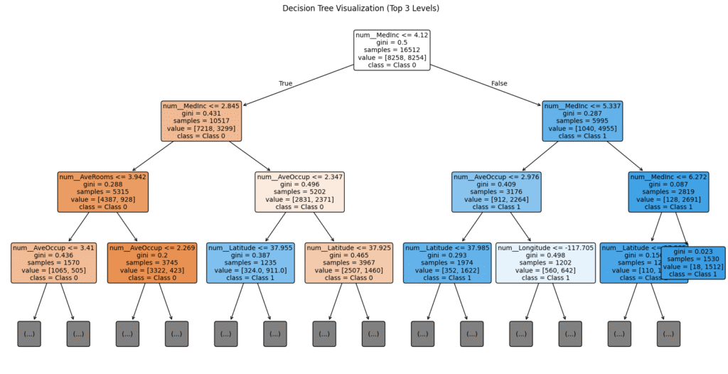
Reading the Node Box:
Each box in the visualization typically tells you:
- Split Condition: e.g.,
age <= 30.5. If true, go left; if false, go right. gini/entropy: The impurity of the node. Lower is better.samples: How many training examples reached this node.value: The count of samples for each class in this node (e.g.,[10, 50]).class: The majority class prediction if the tree stopped here.
Tracing Prediction Paths
To understand why a specific instance was classified a certain way, you can retrieve its decision path. This is the sequence of nodes the instance traversed from root to leaf.
# Use the fitted preprocessing step to transform the raw test row
# into the numeric feature space expected by the tree object.
pre = best_pipe.named_steps["preprocess"]
tree = best_pipe.named_steps["model"]
X_test_transformed = pre.transform(X_test)

# Get the decision path for the first test example.
sample_id = 0
sample = X_test_transformed[sample_id:sample_id + 1]
node_indicator = tree.decision_path(sample)
leaf_id = tree.apply(sample)[0]

feature_indices = tree.tree_.feature
thresholds = tree.tree_.threshold

print(f"Prediction path for sample {sample_id}:")
# `node_indicator` is a sparse matrix containing the visited node ids.
for node_id in node_indicator.indices:
    if leaf_id == node_id:
        print(f"  -> Reached Leaf Node {node_id}")
        continue

    # Retrieve the split rule stored at this internal node.
    feature_idx = feature_indices[node_id]
    threshold = thresholds[node_id]
    feature_name = feature_names[feature_idx]

    # Look up the transformed feature value for this sample.
    val = sample[0, feature_idx]

    threshold_sign = "<=" if val <= threshold else ">"
print(f" Node {node_id}: {feature_name} (= {val:.3f}) is {threshold_sign} {threshold:.3f}")The expected output is a step-by-step trace of the decision path for the specified test sample, showing which nodes were visited and the conditions evaluated at each internal node, culminating in the leaf node reached. This can be invaluable for debugging and explaining individual predictions.
Prediction path for sample 0:
  Node 0: num__MedInc (= 3.153) is <= 4.120
  Node 1: num__MedInc (= 3.153) is > 2.845
  Node 141: num__AveOccup (= 2.755) is > 2.347
  Node 183: num__Latitude (= 33.860) is <= 37.925
  Node 184: num__Longitude (= -117.870) is <= -117.805
  Node 185: num__AveOccup (= 2.755) is <= 3.214
  Node 186: num__Latitude (= 33.860) is <= 34.475
  Node 187: num__AveOccup (= 2.755) is <= 2.786
  Node 188: num__HouseAge (= 19.000) is > 18.500
  Node 190: num__HouseAge (= 19.000) is <= 43.500
  -> Reached Leaf Node 191
Note: When using a
Pipeline,X_testabove needs to be the output ofpreprocess.transform(X_test), or you must manually map the feature values back to the raw input.
7. From-Scratch Training: The Algorithmic Skeleton
Understanding the recursion clarifies what the library is doing and why certain hyperparameters help.
7.1 High-Level Pseudocode
At each node:
- If a stopping condition holds, return a leaf.
- For each feature, enumerate candidate splits.
- Pick the split with best impurity reduction.
- Recurse to build left and right subtrees.
Pseudo-implementation outline:
build_tree(S):
  if stopping_condition(S):
    return Leaf(prediction_from(S))

  best_split = argmax_split(score(S, split))
  S_left, S_right = partition(S, best_split)

  return Node(
    split=best_split,
    left=build_tree(S_left),
    right=build_tree(S_right)
)7.2 Practical Stopping Conditions
- Maximum depth reached.
- Node has fewer than
min_samples_splitsamples. - Impurity reduction is below a threshold (
min_impurity_decrease). - Node is already pure (all labels identical).
7.3 Why Local Decisions Can Miss Better Global Trees
A useful mental warning is that the best first split is not always the first split that leads to the best final tree. Sometimes a root split that looks only moderately helpful opens the door to two very clean splits one level deeper. A greedily chosen alternative may look slightly better immediately, yet leave both child nodes hard to separate later.
This is exactly the kind of trade-off that greedy algorithms ignore. They optimize the next move, not the entire game tree of future moves. That does not make the algorithm bad; it makes the algorithm practical. But it is an important reason to treat a learned tree as one plausible explanation of the data rather than the unique true structure hiding inside it.
8. Practical Tips and Best Practices
This section focuses on the mistakes that repeatedly show up in real projects, and the habits that prevent them.
The unifying theme is simple: trees make it very easy to fit signal, but they also make it very easy to fit artifacts. Good tree practice is mostly about distinguishing the two.
Start With a Regularized Tree
Avoid training an unconstrained tree and hoping it generalizes.
Good starting points:
- Use
min_samples_leafin the range 10–100 for medium datasets (then tune). - Set
max_depthto a modest value (for example 4–10) if interpretability matters. - Consider pruning (
ccp_alpha) when you want a smaller, more stable tree.
Use the Right Metrics
- For imbalanced classification, accuracy can be misleading.
- Prefer
f1,f1_macro,balanced_accuracy, PR-AUC, or cost-sensitive evaluation depending on the problem.
Handle Class Imbalance Deliberately
Options:
- Set
class_weight="balanced". - Use stratified splits and cross-validation.
- Consider threshold tuning on predicted probabilities.
Control Data Leakage
Common leakage patterns with trees:
- Using future information in time series features.
- Encoding categories using the full dataset instead of fitting encoders inside a pipeline.
- Doing imputation outside cross-validation.
The pipeline pattern in Section 6 avoids many leakage issues.
Expect High Variance, Especially on Small Data
Trees are high-variance models. If performance fluctuates across folds, this is expected.
Practical responses:
- Increase
min_samples_leaf. - Reduce
max_depth. - Prefer ensembles (random forests, gradient boosting) when interpretability of a single tree is not required.
Interpret Feature Importance Carefully
Standard tree feature importance is based on impurity reduction and can be misleading:
- It can over-emphasize high-cardinality features.
- It can understate correlated features (if one feature is selected, its correlated partner might be ignored, appearing unimportant).
MDI (Mean Decrease in Impurity):
The default feature_importances_ attribute in scikit-learn calculates the total reduction in impurity (weighted by the probability of reaching that node) brought by that feature. It is fast but biased.
Permutation Importance
Permutation importance measures how much the model’s performance drops when a feature is randomly shuffled. This breaks the relationship between the feature and the target, revealing the feature’s true contribution to the model’s predictive power.
from sklearn.inspection import permutation_importance

# Calculate permutation importance on the test set
# n_repeats=10 means we shuffle each feature 10 times to get stable stats
result = permutation_importance(
    best_pipe, X_test, y_test, n_repeats=10, random_state=42, n_jobs=-1
)

# Sort and print features by importance
sorted_idx = result.importances_mean.argsort()[::-1]

print("Permutation Importance:")
for i in sorted_idx:
    print(f"{X_test.columns[i]}: {result.importances_mean[i]:.4f} +/- {result.importances_std[i]:.4f}")

# Expected output:
#     Permutation Importance:
#     Latitude: 0.1821 +/- 0.0053
#     Longitude: 0.1668 +/- 0.0041
#     MedInc: 0.1558 +/- 0.0057
#     AveOccup: 0.0575 +/- 0.0029
#     AveRooms: 0.0147 +/- 0.0016
#     HouseAge: 0.0090 +/- 0.0015
#     Population: 0.0008 +/- 0.0005
# AveBedrms: -0.0004 +/- 0.0008SHAP (SHapley Additive exPlanations)
For the gold standard in interpretability, SHAP values provide local (per-prediction) and global explanations. They consistently handle correlated features and allocate credit fairly (“game theory” optimal). While external to scikit-learn, the [shap](https://shap.readthedocs.io/en/latest/) library has specialized, high-speed explainers for trees (TreeExplainer).
No importance method should be interpreted in isolation. A feature can appear important because it is genuinely causal, because it acts as a proxy for another variable, or because the dataset contains leakage. Importance tells you what the model used, not automatically what the world works through.
If interpretability is a primary goal, also consider:
- Inspecting representative decision paths (per-example explanations).
- Calibrating predicted probabilities if you plan to use them as probabilities (trees are often poorly calibrated).
9. Common Failure Modes (Debugging Checklist)
- Training score is near-perfect but test score is poor: overfitting; tighten
min_samples_leaf, add pruning. - Tree is extremely deep: add
max_depthor raisemin_samples_leaf. - Model refuses to fit due to NaNs: add imputers in a pipeline.
- Suspiciously good cross-validation: re-check leakage (time splits, encoders, target leakage).
- Rules look unintuitive: review feature definitions, binning/encoding, and target quality.
- One categorical feature dominates splits: check cardinality, encoding choice, and leakage.
- Training is unexpectedly slow: reduce feature count, set
max_depth, or sample candidates via a smallermax_features(if supported).
10. Decision Trees in the Bigger Picture
A single decision tree is a strong educational model and a good baseline. However, for many production tabular problems, the best performance comes from tree ensembles:
- Random forests: reduce variance by averaging many trees trained on bootstrapped samples.
- Gradient boosting (XGBoost, LightGBM, CatBoost): sequentially build trees to correct errors, often state-of-the-art on tabular data.
If you need interpretability, you can still use ensembles with tools such as partial dependence, SHAP, or monotonic constraints (depending on the library), but a single tree remains the most straightforward for rule-based explanations.
A Brief Family Tree: ID3, C4.5, and CART
It is helpful to know that “decision tree” is a family name, not one single algorithm.
- ID3 popularized top-down tree induction using information gain, mainly for categorical features.
- C4.5 extended ID3 with improvements such as gain ratio, handling of continuous features, and pruning.
- CART (Classification and Regression Trees) standardized binary splits and became especially influential in modern libraries.
Most practitioners using scikit-learn are effectively using the CART style of tree induction. That is why binary splits, Gini impurity, and cost-complexity pruning show up so often in modern tutorials.
11. Summary
- A decision tree learns a sequence of data-driven questions that recursively partition the input space.
- In classification, the quality of a split is typically measured by impurity reduction through entropy or Gini; in regression, it is measured by reduction in variance or squared error.
- A tree is expressive because it can model interactions and nonlinear threshold effects, but it is unstable because training is greedy and small changes in data can alter early splits.
- Regularization matters. Controls such as
min_samples_leaf,max_depth, andccp_alphaare not optional details; they are what turn a memorizing tree into a model that has a chance to generalize. - Proper preprocessing and evaluation still matter: imputation, categorical handling, leakage prevention, and the right metric can matter as much as the split criterion itself.
- A single tree is often best viewed as an interpretable baseline and a conceptual foundation for stronger ensemble methods.
The main idea to keep in mind is simple: a decision tree turns prediction into a sequence of local questions. Its power comes from recursively carving the input space into simpler regions. Its weakness comes from making those cuts greedily, which means it can overreact to noise when left unconstrained. Once that mental model is clear, the rest of the algorithm, from impurity measures to pruning to ensembles, becomes much easier to understand.

Happy is a seasoned ML professional with over 15 years of experience. His expertise spans various domains, including Computer Vision, Natural Language Processing (NLP), and Time Series analysis. He holds a PhD in Machine Learning from IIT Kharagpur and has furthered his research with postdoctoral experience at INRIA-Sophia Antipolis, France. Happy has a proven track record of delivering impactful ML solutions to clients.
Subscribe to our newsletter!