From Tokens To Vectors: Demystifying LLM Embedding For Contextual Understanding

The embedding layer in LLM is a critical component that maps discrete input tokens (words, subwords, or characters) into continuous vector representations that the model can process effectively.
In this article, we will delve into the intricacies of LLM embedding layers, focusing on token and positional embeddings, which together form the fundamental input presentation for these models.

The embedding layer maps words or subwords to dense vectors in a high-dimensional space. These vectors encode semantic and syntactic information, enabling the model to comprehend the contextual and relational aspects of language.

Architecture of the Embedding Layer

The embedding layer is essentially a lookup table implemented as a matrix. Its main components are:

a. Token Embedding: Capturing Semantic Meaning

Embedding Matrix Dimensions: \( V \times d \), where:
- \( V \) = Vocabulary size (number of unique tokens)
- \( d \) = Embedding dimension (typically a hyperparameter)
Each row in the matrix corresponds to a vector representation of a token in the vocabulary.
Given an input token’s index \( i \), the embedding layer retrieves the \( i \)-th row of the embedding matrix as the token’s embedding vector.
Embedding matrix is learned during training of the model through a concept called weight tying.

b. Positional Embedding

While token embeddings capture the semantic meaning of words, positional embeddings provide information about the relative or absolute position of tokens within a sequence.
These are typically added to (sometimes concatenated) with token embeddings.
Position embeddings can be learned or fixed (e.g., sinusoidal embeddings).
- If learned, it’s a matrix \(( L \times d )\), where \( L \) is the maximum sequence length.
- If fixed (e.g., sinusoidal), the embeddings are computed algorithmically.

c. Input Representation

Token and positional embeddings are typically combined element-wise to form the final input representation for the LLM. This combined representation captures both the semantic meaning and the sequential order of the input text, enabling the model to effectively process and understand natural language.
For each token in a sequence:
\[
\text{Input Representation} = \text{Token Embedding} + \text{Positional Embedding}
\]

How Embedding Parameters Are Learned

The parameters of the embedding matrix are learned during the training process, using the same backpropagation mechanism that updates other model weights. Here’s how this works:

Forward Pass

Input Tokenization: Text data is tokenized into token IDs. Tokenization methods:
- Word-level: Breaks input into words (rare for LLMs).
- Subword-level: Uses subword units (e.g., Byte Pair Encoding (BPE), WordPiece).
- Character-level: Breaks into individual characters (less common for LLMs).
- Word Embeddings: Pre-trained embeddings like Word2Vec, GloVe.
Embedding Lookup: Each token ID is mapped to its corresponding row in the embedding matrix. The positional embeddings are retrieved or computed for the positions.
Vector Representation: The embedding vectors are formed for each token by adding (more common) or concatenating token embedding and positional embedding.
Processing by Transformer Layers: These embeddings are processed by subsequent layers (e.g., attention layers, feedforward layers) to compute predictions.

Backward Pass

Loss Computation: The model compares predictions to the ground truth and computes a loss (e.g., cross-entropy loss for language modeling).
Gradient Computation: Gradients are computed for all model parameters, including the embedding matrix, with respect to the loss.
Parameter Updates:

Gradients are used to update the embedding matrix entries via stochastic gradient descent (SGD) or its variants (e.g., Adam).

For example, if the \( i \)-th token is used in training, only the corresponding row of the embedding matrix (and the gradients for it) will be updated in that step.

4. Example

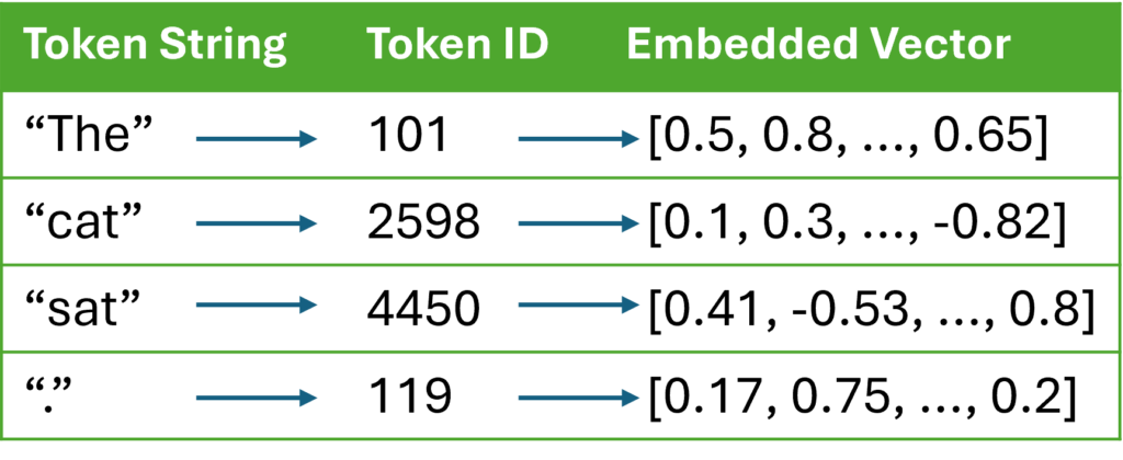
Let’s consider training a transformer-based LLM on the sentence "The cat sat.".

Input Steps:

Tokenization:
- Sentence: "The cat sat." Tokens: ["The", "cat", "sat", "."] Token IDs: [101, 2598, 4450, 119]
Token Embedding Lookup:
- Retrieve embeddings for each token ID from the embedding matrix \(( V \times d )\).
  For example:
  Embedding(101) = [0.5, 0.8, ...] Embedding(2598) = [0.1, 0.3, ...]
Positional Embedding:
- Assume \( \text{Position 0} = [0.01, 0.02, …] \), \( \text{Position 1} = [-0.03, 0.05, …] \).
Summation:
- Input Vector 0 = Embedding(101) + Position(0) Input Vector 1 = Embedding(2598) + Position(1)

Special Techniques for Learning Embeddings

Pre-training:
- Embeddings are initially trained on large corpora using objectives like:
  - Masked language modeling (e.g., BERT).
  - Causal language modeling (e.g., GPT).
- This helps embeddings capture rich semantic relationships.
Regularization:
- Dropout or weight decay is applied to embedding layers to prevent overfitting.
- Techniques like subword tokenization (e.g., Byte-Pair Encoding, WordPiece) are used to keep the vocabulary size manageable.
Dynamic Tokenization:
- Models like T5 and GPT handle subwords, ensuring embeddings can generalize across rare and frequent tokens.

Benefits of Embedding Layer

Compact Representation: Converts sparse token IDs into dense vectors.
Semantic Understanding: Embeddings capture token meaning and relationships.
Flexibility: Positional embeddings encode sequence order for transformers.

Key Advantages of Positional Embeddings:

Handling Variable-Length Sequences: Positional embeddings enable the model to process sequences of varying lengths.
Capturing Long-Range Dependencies: Sinusoidal functions can capture long-range dependencies between tokens, which is essential for understanding complex language patterns.
Generalization to Unseen Sequences: Positional embeddings can generalize to unseen sequences, as they are based on mathematical functions rather than learned parameters.

Properties of Embeddings

Embeddings capture semantic relationships. For instance:
Word analogies: \( \text{vec(“king”)} – \text{vec(“man”)} + \text{vec(“woman”)} \approx \text{vec(“queen”)} \).
Zero-shot learning is enabled in LLMs partly due to the generalization power of these embeddings.

In summary, the embedding layer is a parameterized lookup table learned via backpropagation during model training, capturing semantic properties of language through pre-training and fine-tuning. Its architecture and learning process are foundational to the performance and flexibility of LLMs.