Logistic Regression is one of the simplest and most widely used building blocks in machine learning. In this article, we will start with an intuitive picture of what it does, connect that to the underlying mathematics, and then map those ideas directly into a PyTorch implementation.
The goal is that by the end, Logistic Regression in PyTorch feels less like a mysterious “model” and more like a small, transparent computational graph that you could extend into deeper neural networks.
1. What Problem Does Logistic Regression Solve?
Logistic Regression is a fundamental algorithm for binary classification. Whereas Linear Regression predicts continuous values (such as house prices), Logistic Regression predicts the probability that an instance belongs to a specific class (such as “Spam” or “Not Spam”).
Instead of outputting a raw number that can range from negative to positive infinity, we want an output between 0 and 1. This lets us interpret the result as a confidence score. For example, a prediction of 0.95 means the model is 95 percent confident the input belongs to the positive class.
At inference time, we typically convert this probability into a hard decision by applying a threshold, for example classifying as Class 1 if the probability is greater than 0.5 and Class 0 otherwise.
Visualizing the Transformation
Standard linear models produce straight lines in the input space. If we used a straight line directly for classification, predictions could far exceed 1 or drop below 0, which does not make sense for probabilities.
To fix this, we apply a transformation function that “squashes” the linear output into the range \([0, 1]\). This function is called the Sigmoid function.
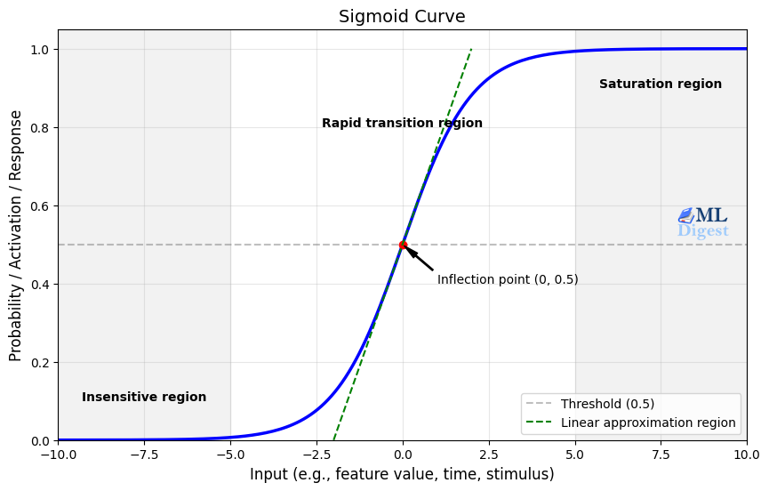
The Sigmoid curve takes any real-valued number and maps it to a value between 0 and 1.
You can think of the Sigmoid as a smooth step function: to the left, the model is very confident it is Class 0; to the right, it is very confident it is Class 1; and in the middle, it is uncertain.
2. The Mathematical Engine
With the core intuition established, let us look under the hood. Logistic Regression is essentially Linear Regression whose output is passed through a Sigmoid activation function.
2.1 The Linear Step
First, the model computes a linear combination of the inputs. If we have input features \(x\), weights \(w\), and a bias \(b\), the linear output \(z\) is
$$ z = w \cdot x + b $$
2.2 The Activation Step (Sigmoid)
Next, we pass \(z\) through the Sigmoid function, denoted as \(\sigma(z)\). This function “squashes” the output to be between 0 and 1:
$$ \hat{y} = \sigma(z) = \frac{1}{1 + e^{-z}} $$
Here, \(\hat{y}\) represents the estimated probability that the input belongs to the positive class (Class 1).
2.3 The Cost Function (Binary Cross Entropy)
How do we train this model so that its probabilities match the data? In Linear Regression, we often minimize the Mean Squared Error (MSE), which measures squared distances between predictions and targets. For classification, however, “distance” is less meaningful than likelihood and confidence.
For Logistic Regression, we use Binary Cross Entropy (BCE) loss, also known as the negative log-likelihood for Bernoulli outcomes. Intuitively, BCE measures how surprised the model is by the true labels, given the probabilities it predicted.
You can think of BCE as a strict teacher who penalizes you based on how confident you were in the wrong answer:
- If the true label is 1 and you predict 0.9 (confident and correct), the penalty is small.
- If the true label is 1 and you predict 0.1 (confident but wrong), the penalty is very large.
The formula for the loss \(L\) for a single example is
$$ L = – \left[ y \log(\hat{y}) + (1 – y) \log(1 – \hat{y}) \right], $$
where \(y\) is the actual label (0 or 1) and \(\hat{y}\) is our prediction.
For a dataset with\( N\) examples, we usually take the average loss
$$ \mathcal{L}(w, b) = \frac{1}{N} \sum_{i=1}^{N} – \left[ y_i \log(\hat{y}_i) + (1 – y_i) \log(1 – \hat{y}_i) \right]. $$
Minimizing this loss with respect to \(w\) and \(b\) is equivalent to maximizing the likelihood of the observed labels under a Bernoulli model with probabilities \(\hat{y}_i\).
3. Optimizing Logistic Regression
To train the model, we adjust \(w\) and \(b\) to minimize the Binary Cross Entropy loss. This is done using gradient-based optimization.
At a high level, the training process repeats the following steps:
- Forward pass: Compute predictions \(\hat{y}_i\) for the current parameters.
- Compute loss: Evaluate \(\mathcal{L}(w, b)\) on the training data.
- Backward pass: Use backpropagation to compute gradients \(\partial \mathcal{L} / \partial w\) and \(\partial \mathcal{L} / \partial b\).
- Parameter update: Adjust \(w\) and \(b\) in the opposite direction of the gradients (for example using Stochastic Gradient Descent).
In PyTorch, most of this machinery is handled for you. You define the computation for the forward pass, and PyTorch automatically builds the corresponding backward pass.
4. Code Implementation: The “Easy Button” vs. The “Engine Room”
Before we build the engine from scratch in PyTorch, let us look at the “easy button.” In the Python ecosystem, scikit-learn is the industry standard for classical machine learning. It abstracts away the calculus and optimization, giving you a robust model in a handful of lines of code.
4.1 The Scikit-Learn Approach
If you just need a logistic regression model for a tabular dataset, this is often the best tool for the job. It uses highly optimized C and Fortran solvers under the hood and provides a familiar, estimator-style interface.
from sklearn.linear_model import LogisticRegression
from sklearn.metrics import accuracy_score

# 1. Initialize the model
# sklearn handles the optimizer (solver) and loss function internally
clf = LogisticRegression(random_state=42)

# 2. Train the model (Fit)
# Note: sklearn works natively with numpy arrays
clf.fit(X_numpy, y_numpy)

# 3. Make predictions
y_pred_sklearn = clf.predict(X_numpy)

# 4. Evaluate
acc = accuracy_score(y_numpy, y_pred_sklearn)
print(f"Sklearn Accuracy: {acc:.4f}")This approach is ideal when you want a strong, battle-tested baseline quickly and do not need to customize the internals of the model.
4.2 Why Build it in PyTorch? (Comparison)
If scikit-learn is faster to write and often faster to run on small data, why use PyTorch? The key reasons are control, scale, and context.
| Feature | Scikit-Learn (The Sports Car) | PyTorch (The Engine Block) |
|---|---|---|
| Coding philosophy | “Black box”: You focus on the input and output. The math happens inside pre-compiled C and C++ routines. | “Glass box”: You define the math explicitly. You see the gradients flow and you control the update step. |
| Inference and scale | CPU bound: Excellent for datasets that fit in RAM; inference is fast for single rows but less flexible for massive parallelism. | GPU accelerated: PyTorch tensors can live on the GPU. For very large datasets, PyTorch can parallelize operations across thousands of CUDA cores. |
| Data handling | In-memory: Typically expects the whole dataset (or chunks you manage manually) in memory. | Mini-batching: Natively supports streaming data in small batches. You can train on datasets larger than RAM. |
| Purpose | Production ML for classical models: Best for standalone tabular tasks and quick baselines. | Deep learning foundation: Logistic Regression in PyTorch is just a neural network with zero hidden layers. Understanding this structure is a gateway to CNNs, RNNs, and Transformers. |
In other words, scikit-learn is the high-level tool you reach for when you want results quickly, while PyTorch is what you reach for when you want to understand, customize, and ultimately build more complex architectures.
5. Building Logistic Regression in PyTorch
Let us translate this theory into a working PyTorch model. We will create a simple dataset, build the model, and train it.
Step 1: Setup and Data Generation
We will generate two clusters of data points to simulate a binary classification problem.
import torch
import torch.nn as nn
import torch.optim as optim
import numpy as np
import matplotlib.pyplot as plt
from sklearn.datasets import make_blobs

# 1. Generate Synthetic Data
# We create 1000 points centered around two clusters
n_samples = 1000
X_numpy, y_numpy = make_blobs(n_samples=n_samples, centers=2, n_features=2, random_state=42)

# Convert to PyTorch Tensors
# Note: PyTorch expects float32 for weights and inputs
X = torch.tensor(X_numpy, dtype=torch.float32)
y = torch.tensor(y_numpy, dtype=torch.float32).view(-1, 1) # Reshape to column vector

print(f"Input shape: {X.shape}")
print(f"Labels shape: {y.shape}")Step 2: Defining the Model
In PyTorch, we define models by subclassing nn.Module. Conceptually, our Logistic Regression model is a single linear layer followed by a Sigmoid.
The Sigmoid activation can be applied during the forward pass (as in this example) or be absorbed into the loss function via BCEWithLogitsLoss, which is numerically more stable for extreme values.
class LogisticRegressionModel(nn.Module):
    def __init__(self, input_features):
        super(LogisticRegressionModel, self).__init__()
        # A single linear layer: z = wx + b
        self.linear = nn.Linear(input_features, 1)

    def forward(self, x):
        # We return the linear output (logits) directly.
        # We will apply Sigmoid later or use a loss function that handles it.
        outputs = self.linear(x)
        return torch.sigmoid(outputs)

# Initialize the model
input_features = 2  # We have x1 and x2 coordinates
model = LogisticRegressionModel(input_features)Step 3: Loss and Optimizer
We use BCELoss (Binary Cross Entropy Loss) because our model outputs probabilities via torch.sigmoid. We will use Stochastic Gradient Descent (SGD) to update our weights.
# Loss function
criterion = nn.BCELoss()

# Optimizer (Stochastic Gradient Descent)
learning_rate = 0.01
optimizer = optim.SGD(model.parameters(), lr=learning_rate)Step 4: The Training Loop
This is the heartbeat of the process. For every epoch (a full pass over the dataset), we
- Perform a forward pass: Make predictions with the current parameters.
- Compute the loss: Measure how far the predictions are from the true labels.
- Perform a backward pass: Let PyTorch compute gradients of the loss with respect to each parameter.
- Update the weights: Use the optimizer to move parameters in the direction that reduces the loss.
num_epochs = 100
losses = []

for epoch in range(num_epochs):
    # 1. Forward pass
    y_predicted = model(X)

    # 2. Compute loss
    loss = criterion(y_predicted, y)
    losses.append(loss.item())

    # 3. Backward pass
    loss.backward()

    # 4. Update weights
    optimizer.step()

    # 5. Zero gradients for the next step
    optimizer.zero_grad()

    if (epoch+1) % 10 == 0:
print(f'Epoch: {epoch+1}, Loss: {loss.item():.4f}')Step 5: Evaluation
Let us see how well our model learned to separate the two clusters. We convert the probabilities into binary predictions (0 or 1) using a threshold of 0.5.
with torch.no_grad():
    y_predicted = model(X)
    # Convert probabilities to 0 or 1
    y_predicted_cls = y_predicted.round()

    # Calculate accuracy
    accuracy = y_predicted_cls.eq(y).sum() / float(y.shape[0])
print(f'Accuracy: {accuracy:.4f}')6. Summary
We have successfully built a Logistic Regression model from scratch in PyTorch. Here is what we covered:
- The Concept: Logistic Regression predicts probabilities for binary classification tasks.
- The Math: It uses the Sigmoid function to squash linear outputs into probabilities and Binary Cross Entropy to measure error.
- The Code: We implemented a custom
nn.Module, defined the optimization loop, and achieved high accuracy on a synthetic dataset.
This fundamental block forms the basis of much deeper neural networks. A neural network is, in many ways, just layers of these logistic regression units stacked together, learning increasingly complex patterns.

Silpa brings 5 years of experience in working on diverse ML projects, specializing in designing end-to-end ML systems tailored for real-time applications. Her background in statistics (Bachelor of Technology) provides a strong foundation for her work in the field. Silpa is also the driving force behind the development of the content you find on this site.
Subscribe to our newsletter!