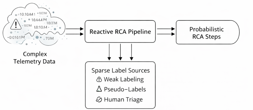
1. Problem framing (what “reactive RCA” means)
Imagine you are a doctor in a busy emergency room. A patient (the SmartCam device) arrives with sudden, severe symptoms (a failure trigger, like a frozen video stream). You do not have time to monitor them for days; you need to diagnose them right now based on their immediate vitals (telemetry) and medical history (firmware/driver versions). This is the essence of Reactive Root Cause Analysis (RCA).
Failures in SmartCam devices are rare (<1%), but when they occur, they disrupt critical workflows like video conferencing or streaming. Unlike silent backend failures, these are highly visible and frustrating user experiences. To solve this, we must build a system that bridges the gap between raw data and actionable engineering insights.
When a failure happens, the device emits a high-dimensional telemetry “trail”: USB power transitions, frame timing instability, error codes, driver resets, lighting estimate anomalies, and crash fingerprints.
Reactive RCA means the system only activates after a failure is detected. Its goal is to act as an automated triaging doctor. Given a short time window of telemetry around the failure, it must produce:
- A ranked list of likely root causes (e.g., firmware defect, driver incompatibility, OS regression, power management issue).
- Actionable evidence for each hypothesis (log signatures, metric deviations).
- Recommended next actions (e.g., collect dump, roll back driver, disable selective suspend).
The mental model is triage:
- Input: A patient (device) arrives with symptoms (failure trigger).
- Process: Collect vitals (opentelemetry) and history (firmware/driver versions).
- Output: A provisional diagnosis with confidence scores and a treatment plan.
- Feedback: Confirmed outcomes (e.g., “driver rollback fixed it”) become labels for future learning.
The central design challenge is that correlation is cheap, but causality is expensive:
- Confounding: OS and driver versions are strongly confounded (updated together).
- Label Sparsity: Most failures are never root-caused manually.
- Distribution Shift: Every firmware release changes the meaning of “normal” metrics.
- Long Tail: Rare, unique failure modes dominate the distribution.
2. Assumptions and constraints
2.1 Assumptions
- Each device has a stable pseudonymous
device_id. - The client uploads telemetry periodically and on failure (buffered if offline).
- A failure trigger event exists, for example: app crash, stream-start failure, sustained frame drop bursts, driver reset, OS camera subsystem error.
- Timestamps have bounded skew, or the ingestion layer can align by
ingest_time. - A subset of failures is deterministically recognisable via crash signatures or error-code patterns.
2.2 Constraints
- Reactivity: produce RCA within minutes after failure telemetry arrives.
- Actionability: outputs must be useful for support and engineers.
- Robustness: tolerate missing data and release-driven distribution shift.
- Privacy/security: minimize PII and treat crash logs as sensitive.
3. Requirements
3.1 Functional requirements
- Ingest telemetry and detect failures.
- For each failure, produce Top-K causes (K=3–5) with calibrated probabilities.
- Attach evidence and recommended actions.
- Support three views:
- per incident RCA
- cohort analytics (by OS/driver/firmware, region, device model)
- release monitoring (regressions after rollouts)
- Capture human feedback and confirmed labels.
3.2 Non-functional requirements
- Reliability: retries, idempotency, backpressure.
- Latency: p95 end-to-end under a few minutes (failure ingest to RCA output).
- Maintainability: versioned telemetry schema, model versioning, reproducible training.
- Explainability: evidence-first output; audit logs for decisions.
3.3 Success metrics
Because labelled data is sparse, measure success with a mix of predictive and operational outcomes:
- Top-K recall on confirmed labels.
- Calibration (ECE / reliability curves).
- Triage efficiency (MTTR reduction, fewer escalations).
- Post-release regression detection lead time.
4. Root cause taxonomy (make the labels precise)
The top-level classes are useful, but they are often too coarse for action. A practical taxonomy is hierarchical and evidence-aligned.
- Software
- Firmware defect (device-side logic, sensor pipeline)
- Driver incompatibility (GPU/USB/camera stack driver interactions)
- OS regression (OS camera subsystem, scheduling, permissions, kernel changes)
- Platform and power
- Power management issue (USB selective suspend, low-power states, power budget)
- Environment
- Environmental condition (low light, flicker, IR interference, motion blur proxy)
- Hardware
- Hardware degradation (sensor aging, connector issues, thermal paste degradation)
- Unknown/other
- Needs investigation (open set)
The key is that each leaf should map to an investigation and a mitigation.
5. System overview and architecture details
To build our automated triage system, we need an architecture that can ingest symptoms, retrieve medical history, and consult multiple specialists (our RCA engines) in real-time.
5.1 Core Components
The overall system is a hybrid pipeline consisting of five main stages:
- Client instrumentation and failure triggers: The device itself detecting that something has gone wrong.
- Ingestion and raw storage: The intake desk where telemetry is securely collected and stored immutably.
- Sessionization and feature building: Organizing the raw data into a coherent “patient history” (feature vector).
- RCA engines: The specialists (rules, retrieval, and probabilistic models) analyzing the features.
- Serving, dashboards, and feedback loop: Delivering the diagnosis and learning from the outcomes.
5.2 High-level dataflow diagram
Let us visualize how data flows through this system. In the diagram below, notice how the raw telemetry is split into three parallel RCA engines. This ensemble approach ensures that if one engine fails to find a pattern, the others might succeed.
graph TD
    subgraph Client
        D[Device Client] -->|Telemetry + Failure Event| IG[Ingestion Gateway]
    end

    subgraph Data_Platform
        IG --> Raw[Event Storage]
        Raw --> Sess[Sessionizer]
        Sess --> Feat[Feature Builder]
    end

    subgraph RCA_Engines
        Feat --> Sig[Engine A: Signatures]
        Feat --> Ret[Engine B: Retrieval]
        Feat --> Prob[Engine C: Probabilistic Model]
    end

    subgraph Serving
        Sig --> Agg[RCA Aggregator]
        Ret --> Agg
        Prob --> Agg
        Agg --> Rep[Incident Report]
        Rep --> Dash[Dashboards/Alerts]
    end

    subgraph Feedback
        Dash -.-> Human[Triage Feedback]
    end
The dataflow consists of three parallel RCA engines:
- Device client emits telemetry and a failure event.
- Ingestion gateway performs auth, rate limiting, and schema validation.
- Events land in event storage (append-only).
- A sessionizer creates “device sessions” and “failure windows”.
- A feature builder produces a feature vector and weak labels (when possible).
- Three engines run in parallel:
- signatures: deterministic matches
- retrieval: nearest historical failures
- probabilistic model: calibrated ranking
- A RCA aggregator combines predictions + evidence into an incident report.
- Dashboards/alerts show spikes by cohort and distribution shift.
- Triage feedback generates high-value labels for retraining.
5.3 Ingestion and storage
- Ingestion endpoint: Validates schema version and required fields; Assigns
ingest_time; Enforces payload limits (crash logs are large). - Storage: Append-only object storage partitioned by day and schema version; Keeps original payload for forensic analysis.
- Schema registry: A versioned telemetry schema with compatibility rules.
- PII and security: Device identifiers hashed with rotating salt; Crash logs scrubbed (tokenization/redaction) before persistent storage.
5.4 Sessionization and failure windows
To accurately diagnose a failure, we cannot just look at the exact millisecond it occurred. We need to understand the context leading up to it. We define a failure instance $i$ as:
$$ i = (device_id, fail_time, fail_type, context) $$
As illustrated in the diagram below, we create multiple time windows around the failure to capture different dynamics. Think of this as looking at the patient’s immediate symptoms, their activities over the last hour, and their general health over the past month:
graph LR
    subgraph Context
        L["Long Window (Days)"]
        M["Medium Window (15m)"]
        S["Short Window (±30s)"]
    end
    t((Failure t))

    S -->|Triggers| t
    M -->|Precursors| S
    L -->|Degradation| M

    style t fill:#f96,stroke:#333
style S fill:#ff9,stroke:#333- Short window: $[t-30\text{s}, t+30\text{s}]$ captures immediate triggers like driver resets, power transitions, or concurrency bugs.
- Medium window: $[t-15\text{min}, t]$ identifies precursor trends such as increasing memory usage, thermal throttling onset, or app usage patterns.
- Long window: last $N$ sessions/days aggregates longitudinal stats to detect hardware degradation (e.g., lens clouding, connector aging) or slow software leaks.
This multi-window design helps distinguish:
- Sudden compatibility regressions (spikes right after upgrade).
- Environmental conditions (lighting estimation instability during event).
- Hardware degradation (slowly increasing frame drops across days).
5.5 RCA output contract
For each failure instance, produce a stable, auditable incident report:
{
  "failure_id": "...",
    "timestamp": "...",
    "device_context": {"device_model": "...", "os_version": "...", "driver_version": "...", "firmware_version": "..."},
  "top_causes": [
     {
        "cause": "DRIVER_INCOMPATIBILITY",
        "prob": 0.42,
        "evidence": [
          {"type": "signature", "id": "dxgk-driver-reset-0x117"},
          {"type": "feature", "name": "usb_selective_suspend_recent", "value": 1},
          {"type": "feature", "name": "os_driver_combo_risk", "value": 0.91}
        ],
        "recommended_actions": ["collect_crash_dump", "suggest_driver_update", "disable_usb_selective_suspend"]
     }
  ],
    "model_version": "rca_2026_02_18",
  "schema_versions": {"telemetry": "v7"}
}Two details matter in practice:
evidencemust be human-actionable (signature IDs, specific error codes, feature names).- The output must support auditing (model version, schema version, feature version if applicable).
6. Data and features
6.1 Telemetry schema (key entities)
- Device metadata (stable or slowly changing):
device_model,camera_sensor_rev,usb_controller_id(if available),age_days_since_first_seen - Software versions:
firmware_version,driver_version,os_version(major/minor/build),app_version - Power and connectivity:
usb_power_state_events(suspend/resume, selective suspend toggles),battery_mode,ac_power - Performance and pipeline health:
frame_rate_target,frame_rate_actual,frame_drop_count,frame_drop_burstiness,queue_depth,processing_latency_ms,cpu_util,gpu_util,thermal_throttling_flags - Perception/environment proxies:
lighting_estimation_mean,lighting_estimation_variance,auto_exposure_iterations,iso_level - Errors and crashes:
error_codes(standardized enum + raw),driver_reset_events,crash_signature_hash,stacktrace_fingerprint
6.2 Feature engineering principles
6.2.1 Make confounders explicit (OS vs driver)
OS and driver versions are dangerous because correlation can masquerade as causation.
Treat versions as first-class structured variables:
- Parse versions into components (major/minor/build) rather than raw strings.
- Create interaction features:
os_major × driver_major,os_build × driver_minor. - Add “upgrade delta” features:
days_since_os_upgradedays_since_driver_upgradechanged_firmware_in_last_k_days
These features support causal interpretation and help the model learn patterns like: “failures spike within 24 hours after driver upgrade on specific OS builds”.
6.2.2 Build shift-robust features (firmware changes meaning)
Firmware releases can change telemetry distributions. Use features that remain meaningful:
- Rank/quantile based features within a release cohort.
- Ratios and normalized deltas (for example, actual fps / target fps).
- Event-driven counts (driver resets, USB suspend cycles) rather than raw continuous metrics.
- Per-release z-scores computed using rolling baselines.
6.2.3 Capture degradation with longitudinal features
Degradation is often slow. Build longitudinal features:
- Trend slope of
frame_drop_rateover last 14 days. - Increase in
sensor_temperatureat equal workload. - Increasing frequency of recoverable errors.
- “Recovery after reboot” indicator (temporary improvement suggests software; persistent signals suggest hardware).
6.3 Data quality checks
- Missingness patterns: missing crash logs should be tracked as a feature and a pipeline warning.
- Clock skew checks: compare client timestamps to ingest time.
- Duplicate event detection and idempotency keys.
- Schema drift detection: new fields or value ranges (per firmware release).
7. RCA engines (multiple perspectives)
No single model is sufficient. The recommended design is an ensemble built from three complementary lenses:
- Deterministic signatures (high precision)
- Similarity-based retrieval (use the past)
- Probabilistic classification (generalization and calibration)
7.1 Engine A: rules and signatures (high precision, low recall)
Maintain a signature library:
- Crash signature hashes mapped to known defects.
- Known driver error codes and OS camera subsystem errors.
- USB power-state oscillation patterns indicating selective suspend issues.
Output of this engine:
- A candidate root cause with high confidence.
- Evidence snippets linking to exact log lines or signature IDs.
This engine is critical early on when labels are sparse.
7.2 Engine B: retrieval (nearest neighbors over failure embeddings)
Idea: Even when labels are sparse, similar failures tend to cluster together. This engine acts as “collaborative filtering” for failures. If a new failure looks exactly like 50 previous failures that were caused by a USB power issue, it is highly probable the new failure shares the same root cause.
Mechanism:
- Embed: Create a compressed vector $z_i$ for each failure instance using:
- One-hot encoded versions.
- Error code embeddings from a pre-trained lookup.
- Summary statistics (means/variances).
- Text embeddings of scrubbed crash signatures (using a small BERT model).
- Index: Store these vectors in an approximate nearest neighbor (ANN) index (e.g., FAISS), keyed by release cohort.
- Retrieve: At inference time, find the top $N=50$ similar historical failures.
- Vote: Aggregate labels from neighbors:
- If neighbors have confirmed root causes, propose the majority class.
- If neighbors cluster in time near a specific release (but have no label), flag as “potential regression”.
To make this concrete, here is how you might implement the retrieval step using Python and the FAISS library. This code demonstrates how we index historical failures and query them when a new failure arrives:
import numpy as np
import faiss

# 1. Define the embedding dimension (e.g., 128 features representing the telemetry)
dimension = 128

# 2. Simulate historical failure embeddings (normally loaded from your data warehouse)
num_historical_failures = 10000
historical_embeddings = np.random.random((num_historical_failures, dimension)).astype('float32')

# 3. Build the FAISS index for fast similarity search (L2 distance)
# Note: IndexFlatL2 performs exact search. For millions of records,
# you would use an Approximate Nearest Neighbor (ANN) index like IndexIVFFlat.
index = faiss.IndexFlatL2(dimension)
index.add(historical_embeddings)
print(f"Total historical failures indexed: {index.ntotal}")

# 4. A new failure occurs, and we embed its telemetry into a vector
new_failure_embedding = np.random.random((1, dimension)).astype('float32')

# 5. Retrieve the top 50 most similar historical failures
k_neighbors = 50
distances, indices = index.search(new_failure_embedding, k_neighbors)

print(f"Retrieved historical failure indices: {indices[0][:5]} ... (showing first 5 of 50)")
print(f"Distances to new failure: {distances[0][:5]} ...")
# Next step: Look up the known root causes for these 50 indices and take a majority vote.Output:
- A probable root cause based on neighbor consensus.
- A list of
similar_incident_idsfor manual review.
7.3 Engine C: probabilistic root cause model
Idea: A calibrated classifier handles complex interactions (e.g., “this failure only happens when lighting < 10 AND driver > v2.1“) that rules and retrieval miss.
7.3.1 Label structure (hierarchical)
Use a hierarchical classifier to improve data efficiency. The model first predicts the broad category (Software vs Hardware), then the specific sub-cause.
- Software -> {Firmware defect, Driver incompatibility, OS regression}
- Platform -> {Power management}
- Environment -> {Low light, Glare}
- Hardware -> {Degradation}
7.3.2 Handling confounding (OS vs driver)
OS versions and driver versions are highly correlated, often leading standard models to blame the “OS” for a driver bug simply because the driver was released alongside that OS update. This is a classic case where correlation masquerades as causation. To mitigate this:
- Stratified training: Perform cross-validation by holding out entire
(OS major, driver major)combinations to ensure the model learns generalized features, not just version IDs. - Counterfactual features: Instead of raw version strings, use relative features:
driver_age_days,is_driver_out_of_policy_for_os,days_since_update. - Causal regularization: Apply penalties similar to Invariant Risk Minimization (IRM): penalize features that have unstable correlations with the target across different environments (OS versions). If a feature is predictive in one OS but not another, its weight should be suppressed.
- Propensity scoring: Train a small model to predict $P(Driver|OS)$. Use the inverse of this probability as a sample weight during training (Inverse Probability Weighting) to upweight rare legitimate combinations and downweight the common co-occurrences. Crucially, you must clip these weights (e.g., cap them at a maximum value) to prevent exploding gradients when $P(Driver|OS)$ is extremely small.
This is not full causal identification, but it reduces the worst failure mode: blaming the OS only because the OS update carried a driver update.
7.3.3 Shift-aware modeling (Mixture-of-Experts)
Firmware releases often change the baseline distribution of telemetry (e.g., a new auto-exposure algorithm changes mean brightness values). A single global model struggles to adapt to these shifts without constant retraining.
Recommended approach:
- Gate by Firmware Line: Use a Mixture-of-Experts (MoE) architecture where the gating network selects an “expert” sub-network based on the firmware version family (e.g., v1.x vs v2.x). This allows the model to learn distinct feature interactions for different firmware generations while sharing lower-level representations.
- Per-cohort Calibration: Apply temperature scaling separately for each release cohort. A model might be overconfident on the stable v1.0 firmware but underconfident on the new v2.0 beta; global calibration would hurt both.
- Drift Detection: Monitor the Kullback-Leibler (KL) divergence of the output distribution per cohort. If the distribution shifts significantly after a release, trigger an alert for “Model Drift”.
To understand the Mixture-of-Experts concept rigorously, let us look at a simplified PyTorch implementation. The gating network acts as a router, deciding which expert is best suited to diagnose the failure based on the input features (which include the firmware version).
import torch
import torch.nn as nn
import torch.nn.functional as F

class FirmwareMoE(nn.Module):
    def __init__(self, input_dim, num_experts, hidden_dim, num_classes):
        super(FirmwareMoE, self).__init__()
        self.num_experts = num_experts

        # The Gating Network decides which expert to trust based on the input
        self.gate = nn.Linear(input_dim, num_experts)

        # The Experts are specialized sub-networks (e.g., one for v1.x, one for v2.x)
        self.experts = nn.ModuleList([
            nn.Sequential(
                nn.Linear(input_dim, hidden_dim),
                nn.ReLU(),
                nn.Linear(hidden_dim, num_classes)
            ) for _ in range(num_experts)
        ])

    def forward(self, x):
        # 1. Calculate gating weights (probabilities for each expert)
        # Shape: (batch_size, num_experts)
        gate_weights = F.softmax(self.gate(x), dim=1)

        # 2. Calculate the output from each expert
        # Shape: (batch_size, num_experts, num_classes)
        expert_outputs = torch.stack([expert(x) for expert in self.experts], dim=1)

        # 3. Combine expert outputs weighted by the gate
        # We expand gate_weights to multiply across the num_classes dimension
        output = torch.sum(gate_weights.unsqueeze(2) * expert_outputs, dim=1)
        return output

# Example usage:
# 16 failures, each with 64 telemetry features
input_features = torch.randn(16, 64)

# Initialize MoE with 3 experts (e.g., for 3 major firmware lines) and 5 root cause classes
moe_model = FirmwareMoE(input_dim=64, num_experts=3, hidden_dim=32, num_classes=5)

# Get the raw logits
logits = moe_model(input_features)

# Apply softmax to get the probabilistic predictions
predictions = F.softmax(logits, dim=1)
print(f"Output shape: {predictions.shape}") # Expected: [16, 5]7.3.4 Open-set behavior (unknown causes)
Some failures will not fit known categories.
- Add an “UNKNOWN/OTHER” class with a thresholding rule.
- Use confidence thresholding or conformal prediction for abstention:
- Confidence thresholding: If the maximum predicted probability is below a threshold $\tau$, abstain and return “needs investigation”.
- Conformal prediction: Construct a prediction set that guarantees a certain confidence level (e.g., 95%). If the resulting set contains multiple classes (indicating high uncertainty) or is empty, abstain and flag for manual review.
7.4 Aggregation logic
Combine engines using a simple, auditable policy:
- If a high-precision signature match exists, it dominates.
- Otherwise, blend retrieval votes and classifier probabilities:
- $p = \alpha p_{model} + (1-\alpha) p_{retrieval}$
- Attach evidence from whichever engine contributed most.
- Always attach release context (recent OS/driver/firmware changes).
8. Learning with sparse labels
Weak supervision
When starting out, you will likely have very few confirmed labels. To overcome this cold-start problem, we can leverage weak supervision. This involves programmatically generating “weak” labels using heuristics and existing knowledge bases. For instance, we can automatically assign labels based on high-precision signature matches, known violations of the hardware compatibility matrix, or deterministic error-code mappings. Additionally, any lab reproductions that can be mapped back to specific incidents serve as excellent weak labels. By using these weak labels, we can bootstrap the initial classifier and then gradually replace them with high-quality, confirmed labels as they become available.
Human-in-the-loop triage
To build a robust dataset over time, it is crucial to integrate human expertise directly into the workflow. By providing a dedicated triage UI, we empower support engineers to review the system’s predictions. This interface should clearly display the top predicted causes, the supporting evidence, and similar historical incidents. Engineers can then confirm the model’s prediction, override it with the correct cause, or mark it as “unknown” if further investigation is needed. Capturing their insights in structured fields creates a continuous, high-quality label stream that is naturally focused on the most valuable and complex failures, such as sudden spikes or regressions.
Semi-supervised learning
Once the model achieves a reasonable level of performance, we can utilize semi-supervised learning to further expand our training set. This technique involves using the model’s own confident predictions on unlabeled data as pseudo-labels. However, this must be done carefully to avoid reinforcing the model’s mistakes. We should only generate pseudo-labels when the model’s calibration is strong and its abstention rate is low. To account for distribution shifts across different hardware or software versions, it is essential to apply per-cohort confidence thresholds rather than a single global threshold.
9. Evaluation strategy
9.1 Offline evaluation
Because failures are rare, use the right metrics:
- Top-K recall (K=3 or 5): The fraction of incidents where the true root cause appears in the top-K ranked predictions. Given label sparsity, this is more forgiving than top-1 accuracy and aligns with the use case (support can investigate a small number of plausible hypotheses).
- Macro-averaged F1 across root causes: Compute precision and recall per root-cause class, then average them equally. This prevents high-frequency causes (for example, “environment”) from dominating the metric and hiding poor performance on rare causes (for example, “hardware degradation”). In a system where certain failure modes are rare but critical, this metric ensures the model learns them well.
- Calibration (expected calibration error, or ECE; reliability plots): A model that outputs $p=0.7$ should be correct approximately 70% of the time. ECE measures this alignment by binning predictions and comparing empirical accuracy within each bin to the predicted probability. Reliability plots visualize this visually. Poor calibration (for example, overconfident predictions) leads to costly interventions on weakly supported hypotheses.
- Abstention-aware utility: Define a custom scoring function that rewards the system for knowing when it does not know. Specifically:
- Award full credit (1.0) for correct top-1 predictions.
- Award partial credit (0.5) if the true cause is in top-K but not top-1.
- Penalize confident incorrect predictions (for example, $-0.5$).
- Award small reward (0.1) for explicit abstention (“needs investigation”) on hard cases.
9.2 Release-aware backtesting
Perform time-split evaluation aligned with releases. Standard random cross-validation will leak future information and give you a false sense of security. Instead, you must simulate the exact conditions the model will face in production.
- Train up to date $T$.
- Test on failures after $T$ where new firmware/driver/OS versions appear.
- Report performance by cohort:
- per OS build
- per driver family
- per firmware major line
This is the closest thing to “future performance” you can measure.
9.3 Confounding stress tests
Specifically test OS-driver confounding:
- Hold out certain OS builds and evaluate generalization.
- Create matched cohorts (same OS, different drivers; same driver, different OS) where possible.
- Evaluate whether root cause attributions flip when only OS changes.
9.4 Online evaluation
- Shadow mode: run model and log outputs without affecting support decisions.
- Compare against human triage outcomes.
- Track operational metrics: MTTR, number of escalations, reproduction rate.
9.5 The censored-label problem and control groups
In reactive RCA, labels are not only sparse, they are sometimes censored by the system itself.
- If the system recommends an action (for example, “roll back driver”, “disable selective suspend”), then the incident may never reach deeper investigation.
- As a result, some root causes remain unknown not because they are rare, but because mitigations prevent confirmation.
A practical mitigation is to use a small, privacy-safe exploration policy:
- Control group incidents
- Randomly sample a small fraction of incidents (for example, 1% to 5%) where the system still provides recommended actions, but also requests a standardized, minimal extra diagnostic payload (for example, an extended crash fingerprint or an additional telemetry window).
- This “buys labels” through better observability, not through user harm.
- Matched-cohort investigations: For a subset of cohorts (OS build, driver family, firmware major), encourage deeper investigation even for incidents that self-resolve, to prevent blind spots.
- Evaluation metric alignment: Track “label acquisition rate” and “time-to-confirmation” in addition to Top-K recall and calibration.
10. Serving and monitoring
10.1 Serving requirements
- Batch + streaming hybrid
- Streaming path for immediate RCA after failure.
- Batch jobs to compute baselines and update drift statistics.
- Latency target: Feature build and inference within minutes after failure telemetry arrives.
- Stability: If a model is unavailable, fall back to rules + retrieval.
- Versioning: Each prediction stores
model_versionandfeature_version.
10.2 Monitoring dashboards
Monitor three layers:
- Data quality: missingness rates, client upload lag, schema errors
- Model health: calibration drift, prediction entropy, abstention rate
- Product health: failure rate (<1% baseline), spike detection by cohort
10.3 Drift and shift detection
Track drift per cohort:
- Population stability index (PSI) for key features.
- Version cohort emergence (new OS build with no prior data).
- Embedding-space shift (retrieval distances increase).
When drift triggers:
- Increase abstention thresholds.
- Trigger retraining jobs.
- Alert engineering if failures spike for a release.
10.4 Alerting and incident response
Define alerts tied to action:
- “OS regression suspected” alert when failure rate spikes after OS rollout and model attribution concentrates on OS regression with high confidence.
- “Driver incompatibility suspected” when compatibility risk features and driver reset signatures dominate.
- “Power management issue suspected” when suspend/resume oscillations precede failures.
- “Hardware degradation suspected” when longitudinal degradation features cross threshold.
Provide a runbook per alert type:
- How to reproduce
- What additional logs to request
- Suggested mitigation steps for users
10.5 Latency budgeting and operational SLOs
The goal is minutes, not milliseconds, but budgets still matter because incident volume can spike during regressions.
One concrete way to keep the system predictable is to allocate an explicit end-to-end budget (example numbers are illustrative):
- Ingestion validation and persistence: 5 to 15 seconds (including queuing).
- Sessionization and feature building: 30 to 90 seconds.
- Parallel inference (signatures, retrieval, model): 10 to 30 seconds.
- Aggregation, evidence packaging, and write-back: 5 to 15 seconds.
This budgeting clarifies where to optimize first. In practice, feature building and retrieval are often the first bottlenecks, not model compute.
10.6 Kill switch, safe mode, and shadow mode
Release-driven shift can produce confident but wrong attributions. Operationally, the system needs a small set of safety controls.
- Safe mode (fallback path)
- A configuration switch that bypasses the probabilistic model and uses signatures + retrieval only.
- Useful when a new firmware line breaks feature semantics or Model Calibration.
- Shadow mode (pre-release validation)
- Run a candidate model version in parallel, logging outputs and calibration metrics without changing the incident report.
- Promote the model only after release-aware backtesting and shadow validation match expectations.
- Per-cohort circuit breakers
- If drift detectors trigger for a cohort, increase abstention thresholds and rely more on signatures until baselines are rebuilt.
10.7 Practical implementation notes
- Start simple: signatures + retrieval + a calibrated gradient boosted model.
- Add hierarchical classification and MoE only once drift becomes the limiting issue.
- Keep the RCA output contract stable so product and support workflows do not churn.
- Make evidence first-class: store feature contributions (for example, SHAP) and signature IDs.

Happy is a seasoned ML professional with over 15 years of experience. His expertise spans various domains, including Computer Vision, Natural Language Processing (NLP), and Time Series analysis. He holds a PhD in Machine Learning from IIT Kharagpur and has furthered his research with postdoctoral experience at INRIA-Sophia Antipolis, France. Happy has a proven track record of delivering impactful ML solutions to clients.
Subscribe to our newsletter!