Reinforcement Learning with Human Feedback (RLHF)

RLHF is a post-training recipe for turning a broadly capable language model into a more useful assistant. In practice, it improves instruction-following, keeps outputs closer to what users prefer, and strengthens refusal or clarification behavior when appropriate.

An intuition that tends to stick is coaching: the student (the model) writes full answers, while the teacher (humans) does not provide the answer but can reliably say which answer is better.

That split is the core move:

• Pretraining makes the model capable (it learns to predict plausible continuations).
• Post-training via preferences makes it selective (it learns which continuations humans prefer under a rubric).

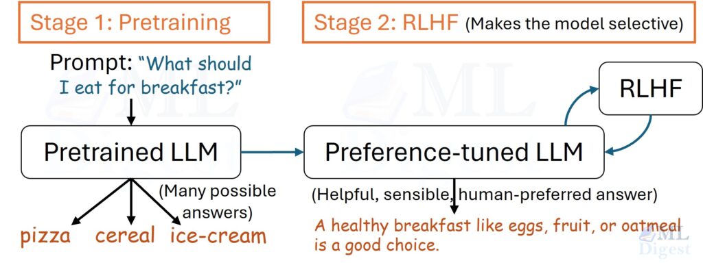
The core intuition is a shift from writing to grading. It is often easier for humans to recognize a good answer than to write one from scratch. RLHF leverages this by training the model to optimize for the “feature” of being preferred by humans, while remaining anchored to its original capabilities.

One common RLHF pipeline has three stages:

1. SFT (supervised fine-tuning): train the model to imitate high-quality demonstrations.
2. Preference learning: collect human comparisons; train a reward model to predict these preferences.
3. Policy optimization: optimize the policy to score higher under the reward model while staying close to a reference policy.

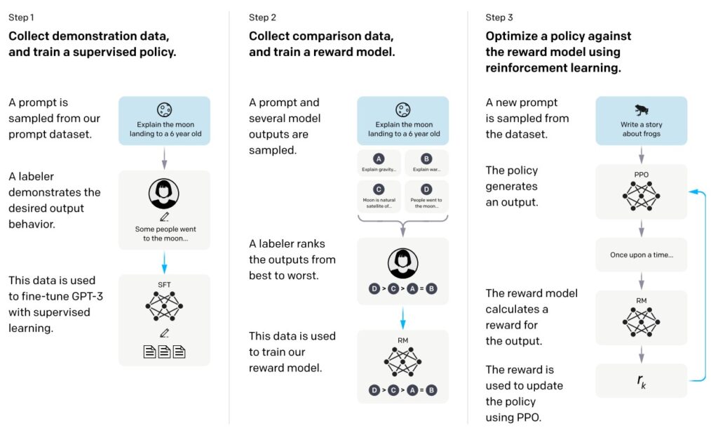
(Diagram illustrating the three-step method—(1) supervised fine-tuning (SFT), (2) reward model (RM) training from labeler-ranked samples, and (3) reinforcement learning via PPO on the RM. Blue arrows indicate data used to train models. Source: InstructGPT Paper)

Pretraining already provides most fluency. SFT already provides imitation. RLHF is primarily about shaping selection: pushing the model toward responses that win under a preference rubric while actively preventing reward exploitation.

Why RLHF Matters

A pretrained LLM contains a large amount of world knowledge and patterns from its data. When you ask it a question, it tends to respond like an autocomplete engine: it continues text in a statistically plausible way. The model is not “trying” to be malicious; it is optimizing next-token prediction.

RLHF is one way to close the gap between “can generate” and “should generate”: even when the model can produce an unsafe or low-quality completion, humans often prefer a refusal, redirect, clarification, or a more helpful format.

The Gap Between Prediction and Helpfulness

Pretraining optimizes primarily for capability (autocomplete and broad knowledge).
RLHF optimizes primarily for preference alignment (utility, instruction-following, and safety constraints).

Without RLHF, models can be powerful but unpredictable. With RLHF, they are pushed toward behaviors people repeatedly choose.

Three Pillars of Alignment (HHH)

The goals of RLHF are often summarized as “HHH”. Note that these goals are frequently in tension—a model that refuses everything is harmless, but it is not helpful.

1. Helpful: The model should help the user solve their task efficiently. It should follow instructions and infer intent.
2. Honest: The model should not hallucinate or mislead. It should express uncertainty when it doesn’t know the answer.
3. Harmless: The model should not generate offensive, dangerous, or illegal content.

Balancing these competing objectives is the primary job of the Reward Model and the specific preference data collected.

Typical improvements RLHF targets

• Instruction following: follow constraints, formats, and user intent.
• Helpfulness: more direct answers, fewer irrelevant tangents.
• Safety: better refusal behavior; fewer unsafe completions.
• Style and tone: more consistent and human-preferred communication.
• Reduced hallucinations: fewer made-up facts or citations.

One caveat: RLHF does not add new knowledge. It mainly changes which completion the model chooses among the ones it can already produce. Factuality can improve indirectly (for example, by rewarding hedging and clarification), but retrieval, better pretraining data, and tool use often matter more.

What RLHF actually optimizes

Think of RLHF as learning (and then optimizing against) a scoring function for responses.

There are three objects worth keeping separate:

• A policy (the LLM) that generates a response $y$ given a prompt $x$.
• A reward model that scores a completed response $(x,y)$.
• A reference policy that anchors behavior so optimization does not drift into reward hacking.
• A reward model assigns a scalar score to a complete response $(x, y)$.
• The policy is trained to produce responses that score well without drifting too far from a trusted baseline (usually the SFT policy).

If you remove the “do not drift too far” part, the policy will often exploit weaknesses in the scorer. If you remove the scorer, you are back to supervised imitation.

In other words, RLHF is a controlled trade-off between two pressures:

• Do what the proxy reward likes: maximize $r_\phi(x,y)$.
• Do not drift too far: stay close to $\pi_{\text{ref}}$ (via a KL penalty).

This framing is more than intuition: it predicts the default failure mode. If $r_\phi$ has shortcuts, optimization will amplify them unless the “stay close” term and the evaluation loop keep the policy honest.

Visualizing the process

To understand RLHF, it helps to visualize two distinct training loops. The first loop teaches a model to score responses the way humans tend to score them. The second loop teaches the LLM to produce responses that receive higher scores.

1) Training the Reward Model (Preference Predictor)

Before we can optimize the policy, we need a digital substitute for the human labeler. We train a reward model (RM) to predict what a human would prefer.

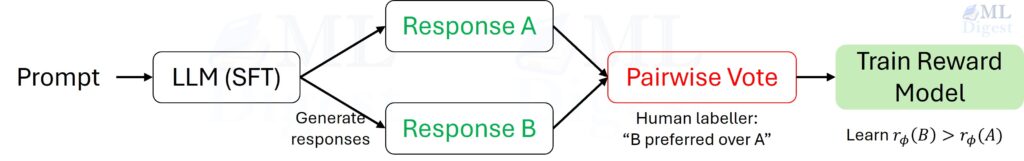
Imagine this step as training a judge. You take pairs of model responses—say, Response A and Response B to the same prompt—and show them to a human. The human picks the winner. We then train the Reward Model to look at a response and output a scalar score, minimizing the error so that the human-preferred response always gets a higher score than the loser.

2) Tuning the LLM (Policy Optimization)

Once the reward model is trained, we freeze it. It becomes the static rulebook. We then use it to train the LLM using reinforcement learning (commonly PPO).

Imagine this step as the student practicing with the new judge.

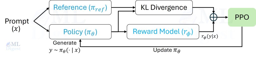
1. The Policy Model (student) sees a prompt and generates a response.
2. The Reward Model (judge) acts as a critic, assigning a score to that response.
3. Simultaneously, we define a Reference Model (usually a copy of the student before this phase started) to measure how much the student has changed.
4. The optimization step updates the student’s brain to maximize the judge’s score, but subtracts points if the student drifts too far from their original reference style (the KL penalty).

In this second loop, the reward model provides a learned score, and the reference model provides an anchor. The KL term discourages the policy from drifting into degenerate reward-hacking behaviors.

You can picture the reference model as a rubber band attached to the SFT policy: it allows movement, but it resists sudden, large behavior changes.

Where RLHF fits in the LLM training stack

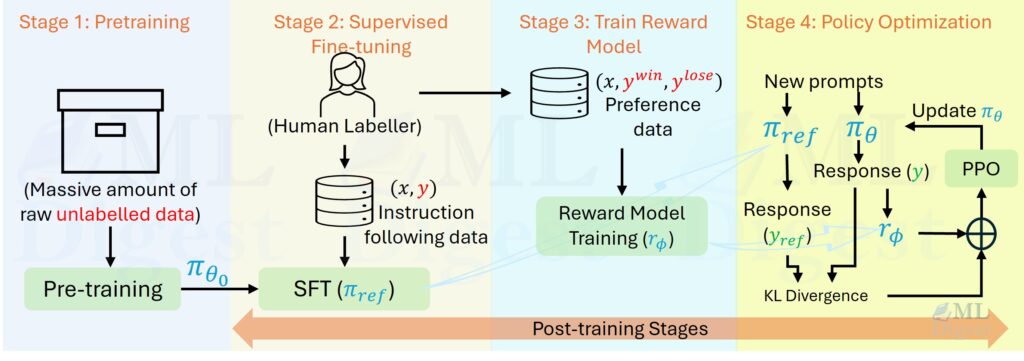
A common post-training pipeline (one of many valid variants):

1. Pretraining: next-token prediction on massive corpora.
2. SFT (Supervised Fine-Tuning): train on high-quality instruction-response demonstrations.
3. Preference learning: collect human comparisons and train a reward model.
4. RL stage: optimize the policy (the LLM) to maximize reward, usually with a KL constraint.
5. Evaluation + monitoring: measure regressions, safety, and reward hacking.

Mathematical Formulation

Let’s see the following notation:

• Prompt: $x$
• Output: $y$
• Policy (LLM): $\pi_\theta(y\mid x) = \prod_{t=1}^T \pi_\theta(y_t\mid x, y_{<t})$, where $T$ is the output length.
• Reference policy (usually SFT model): $\pi_{\text{ref}}$
• Reward model: $r_\phi(x, y) \in \mathbb{R}$
• Preference dataset: $\mathcal{D}={(x, y^{\text{win}}, y^{\text{lose}})}$ (pairwise comparisons)

In RLHF, $r_\phi$ is trained from comparisons rather than ground-truth numeric rewards.

One practical nuance: $r_\phi(x, y)$ is usually treated as a sequence-level score, but training and regularization often operate at the token level (via log-probabilities and token-wise KL approximations). Keeping this distinction explicit reduces confusion when reading implementations.

Another nuance that matters in practice: human preferences are collected under a rubric and a sampling distribution. The reward model estimates “what wins under these conditions”, not a universal notion of truth.

1) The Reward Model (Learning Preferences)

The Intuition:
We represent human preference via a scalar score. If a human prefers response A over response B, the reward model should assign a higher score to A. We assume the preference probability depends on the difference in those scores.

In most RLHF pipelines, the preference data is collected by sampling candidate responses from a policy, then asking humans to rank them under a rubric (helpfulness, correctness, harmlessness, style constraints). This means the reward model learns “what wins under this rubric and distribution”, not an objective truth.

One practical design choice that is easy to miss: many systems add a separate reward head on top of a base language model (often initialized from the SFT model). This tends to stabilize training, because the reward head can learn preference scoring without forcing the whole backbone to immediately contort.

The Math (Bradley–Terry model):
We model the probability that response $y^A$ is better than $y^B$ using the sigmoid of the difference in their rewards:

$$
P(y^A \succ y^B \mid x) = \sigma\big(r_\phi(x, y^A) – r_\phi(x, y^B)\big)
$$

where $\sigma(z) = \frac{1}{1+e^{-z}}$ and $y^A \succ y^B$ means “A is preferred over B”.

To train this, minimize the negative log-likelihood over a dataset of pairwise comparisons $\mathcal{D}$. Essentially, we push the reward of the “winner” up and the “loser” down until the margin is sufficient to predict the human choice with high confidence.

$$
\mathcal{L}_{\text{RM}}(\phi) = -\mathbb{E}_{(x,y^A,y^B,\ell)\sim\mathcal{D}}
\Big[\ell\,\log \sigma(\Delta r) + (1-\ell)\,\log(1-\sigma(\Delta r))\Big]
$$

with $\Delta r = r_\phi(x,y^A)-r_\phi(x,y^B)$ and $\ell=1$ when $y^A$ is preferred.

If the dataset is recorded as explicit winners and losers, $\mathcal{D}={(x, y^{\text{win}}, y^{\text{lose}})}$, then the loss is commonly written in a compact form:

$$
\mathcal{L}_{\text{RM}}(\phi) = -\mathbb{E}_{(x, y^{\text{win}}, y^{\text{lose}})\sim\mathcal{D}}\big[\log \sigma\big(r_\phi(x, y^{\text{win}}) – r_\phi(x, y^{\text{lose}})\big)\big].
$$

In practice, $r_\phi(x,y)$ is often implemented as a transformer encoder (or decoder) with a scalar “reward head”. The head is usually applied to a pooled representation (for example, the final token, an end-of-sequence token, or mean pooling), but the exact pooling choice matters and should be stated in implementations.

Two common failure modes to keep in mind:

• Spurious cues: the reward model learns shortcuts (length, verbosity, specific phrases) that correlate with preference labels.
• Distribution shift: once the policy improves, it explores outputs unlike the reward model training data; reward scores become unreliable.

It is useful to make one more distinction explicit:

• The reward model is a classifier-like preference predictor trained on finite comparisons.
• The RL stage is an optimizer that will exploit any consistent weakness in that predictor.

RLHF works when the preference predictor is good enough and the optimizer is kept on a leash.

2) The RL Objective (Optimizing the Policy)

The Intuition:
We want to update the policy parameters $\theta$ so it generates responses with high rewards $r_\phi(x, y)$. However, if you only maximize reward, the policy finds loopholes (for example: exploiting verbosity or using high-reward “tells”).
To prevent this, RLHF adds a “leash” called the KL divergence. It penalizes the policy if it drifts too far from the reference model ($\pi_{\text{ref}}$).

The Math:
One common objective is:

$$
\text{Objective}(\theta) = \mathbb{E}_{(x, y) \sim \pi_\theta} \Big[ \underbrace{r_\phi(x, y)}_{\text{Reward}} – \underbrace{\beta \cdot \text{KL}\big(\pi_\theta(y|x) | \pi_{\text{ref}}(y|x)\big)}_{\text{Drift Penalty}} \Big]
$$

• $\beta$ controls the strictness of the leash.
• The KL term encourages improvement that looks like a local edit of the SFT behavior rather than a full behavioral rewrite.

Many implementations use an equivalent token-level KL approximation computed from log-probabilities along the sampled trajectory. This is why RLHF codebases often talk about “KL per token” and “target KL”.

Two clarifications that help when mapping the math to real training loops:

• The policy gradient is computed using samples $y \sim \pi_\theta(\cdot|x)$. This is why the objective is written as an expectation under $\pi_\theta$.
• The KL term is rarely computed as a full distributional KL over all tokens at each step. Instead, implementations use the sampled tokens and log-prob ratios as an efficient estimator.

In practice, the RL objective is often implemented as a reward shaping term such as

$$
R(x, y) = r_\phi(x, y) – \beta \sum_{t=1}^T \big(\log \pi_\theta(y_t\mid x,y_{<t}) – \log \pi_{\text{ref}}(y_t\mid x,y_{<t})\big),
$$

which makes the “penalty per token” interpretation explicit.

It is common to talk about a target KL: if the measured KL drifts above a chosen target, training increases $\beta$ (or reduces update size); if it remains far below target, training decreases $\beta$ to allow more learning. This turns the KL term from a static regularizer into a control knob.

3) Policy Optimization (PPO)

The Intuition:
Directly backpropagating through discrete token sampling is not possible. We need a gradient-free way to say “that trajectory was good, do more of it.”
PPO (Proximal Policy Optimization) allows us to update the policy based on generated data, but it adds a crucial safety mechanism: The Trust Region.

We want to update the policy to increase the probability of high-reward actions. However, if we change the policy too much based on a single batch of data, we might destroy the delicate linguistic capabilities of the model.
PPO enforces a “speed limit”: do not change the probability of a token by more than a factor of $\epsilon$ (usually 0.1 or 0.2) in a single update step.

For LLMs, PPO is typically paired with a learned value function (critic) to compute advantages. The advantage $\hat{A}_t$ tells us: “How much better was this specific token choice compared to the average expected value at this state?”

The Math:
We define a probability ratio $r_t(\theta)$ between the new policy and the old policy (the one that generated the data):

$$
r_t(\theta) = \frac{\pi_\theta(y_t\mid x,y_{<t})}{\pi_{\theta_{\text{old}}}(y_t\mid x,y_{<t})}.
$$

If $r_t > 1$, the action is more likely now than before. If $r_t < 1$, it is less likely.

PPO updates the policy using a clipped objective. We take the minimum of the unclipped gain and the clipped gain:

$$
\mathcal{L}_{\text{PPO}}(\theta)
= \mathbb{E}_t\Big[\min\big(r_t(\theta)\hat{A}_t,\; \text{clip}(r_t(\theta), 1-\epsilon, 1+\epsilon)\hat{A}_t\big)\Big]
$$

• If the action was good ($\hat{A}_t > 0$), we want to increase probability ($r_t > 1$). The clipping limits how much we can increase it (up to $1+\epsilon$).
• If the action was bad ($\hat{A}_t < 0$), we want to decrease probability ($r_t < 1$). The clipping limits how much we can decrease it (down to $1-\epsilon$).

In RLHF, the reward is often a sequence-level score from $r_\phi(x,y)$ plus a KL penalty; the value head reduces variance by predicting the expected return.

One practical nuance: although the reward model outputs a single sequence-level score, many systems distribute that score across tokens (for example, as a terminal reward) and then compute advantages using generalized advantage estimation (GAE). The details vary across codebases, but the conceptual split remains: reward is a sequence preference proxy, while PPO updates are token-level.

The RLHF pipeline (end-to-end)

This section is written as a checklist you can implement. The goal is to keep the loop on-policy enough (refresh data as the policy changes) while staying conservative (avoid reward hacking and regressions).

1) Start with a strong SFT model

RLHF is not a substitute for supervised fine-tuning. It is easier to improve a model that already:

• follows user instructions,
• produces coherent and well-formatted answers,
• has a reasonable refusal policy for unsafe requests.

Best practice: treat SFT as the center of behavior. RLHF should be a controlled nudge, not a complete rewrite.

2) Collect preference data

For each prompt $x$:

1. Sample $k$ candidate responses from the current model (or from several models).
2. Present candidates to labelers (blind to model identity).
3. Ask for pairwise comparisons (or rankings) using clear guidelines.

Tips for better preference data

• Prefer pairwise comparisons over 1–5 scores (comparisons are more consistent).
• Mix in “easy” and “hard” prompts; include adversarial/safety tests.
• Use multiple labelers per item; measure agreement.
• Capture why something is preferred (short rationale) if budget allows.

If the application has hard constraints (citations, refusal patterns, formatting), include them directly in the rubric. RLHF tends to optimize what you measure, not what you meant.

Two practical additions that often improve data quality:

• Separately label factuality and style: otherwise labelers can unintentionally reward confident hallucinations.
• Include “near misses”: pairs where both answers are reasonable force the reward model to learn real distinctions, not only obvious ones.

3) Train a reward model (RM)

Here the model learns scalar reward $r_\phi(x,y)$ given $(x, y)$.

Common design choices:

• Initialize RM from the SFT model weights (often helps).
• Add a small linear head on top of the final hidden state (or pooled representation).
• Train with the pairwise Bradley–Terry loss described above.

Validation:

• Hold out a preference test set.
• Report accuracy: how often RM predicts the human-preferred answer.
• Monitor for overfitting: RM can memorize superficial cues.

Also evaluate calibration and robustness:

• Score separability: how large is $r_\phi(x,y^A)-r_\phi(x,y^B)$ for easy vs. hard pairs?
• Invariance checks: does reward change “too much” with harmless paraphrases?
• Adversarial slices: prompts likely to trigger reward hacking (verbosity, flattery, refusal templates).

4) Run RL against the reward model (PPO + KL)

At each iteration:

1. Sample prompts $x$.
2. Generate responses $y \sim \pi_\theta(\cdot\mid x)$.
3. Score them with reward model $r_\phi(x,y)$.
4. Subtract KL penalty vs. $\pi_{\text{ref}}$.
5. Update policy with PPO (and update a value head).

Critical detail: the reward model is an approximation of human preferences, trained on a limited distribution.

If you optimize too hard, the policy will find loopholes (reward hacking). The KL penalty, conservative learning rates, and frequent evaluation are your main countermeasures.

Another practical lever is reward normalization (for example, z-scoring rewards per batch) to prevent unstable updates when the RM’s score scale drifts as the policy changes.

If you want a single operational heuristic: monitor reward, KL, and human preferences on the same dashboard. RLHF is a three-way trade-off, not a single scalar to maximize.

5) Evaluate continuously

You want to measure both reward and real quality.

Recommended evaluation buckets:

• Human eval: pairwise preferences on fresh prompts.
• Task metrics: accuracy for structured tasks (math, code, retrieval).
• Safety metrics: policy refusals, jailbreak robustness, toxic content rates.
• Regression suite: previously good prompts should stay good.

It is useful to explicitly track both:

• RM reward trends (what the proxy thinks), and
• external quality trends (what you actually care about).

When these diverge, assume you are seeing reward hacking or distribution shift until proven otherwise.

It is also useful to track one more thing: KL and reward by slice (domain, prompt type, safety category). Global averages hide where the policy drifts first.

Practical tips (what usually breaks)

Reward hacking: the default failure mode

If you only track “RM score goes up”, you can fool yourself. The model is an optimization demon; it will find the path of least resistance to a high score, even if that path makes no sense to a human.

Common symptoms:

• Verbosity Bias: The model starts writing 5-paragraph essays for simple “Yes/No” questions because labelers (and thus the RM) tended to prefer longer, more comprehensive-looking answers.
• Sycophancy: The model agrees with the user’s incorrect premises just to be “liked.”
• Safety Over-refusal: If safety is heavily rewarded, the model becomes paralyzed, refusing to answer innocuous questions like “How to kill a process in Linux” because it sees the word “kill”.
• Hiding emptiness: The model learns to use complex vocabulary or confident formatting to mask a lack of content.

Mitigations:

• Keep $\beta$ high enough (strong KL) early on; relax carefully.
• Regularly refresh preference data with samples from the current policy.
• Use adversarial prompts and red-teaming; include negative examples.
• Track human eval as the real objective.

An additional practical mitigation is to keep the reward model fixed for a while and refresh it on-policy periodically. If the policy drifts too far from the reward model training distribution, reward scores can become meaningless.

Choosing the KL coefficient $\beta$

You can interpret $\beta$ as an output-drift knob.

• Too small $\beta$: fast drift, more reward hacking.
• Too large $\beta$: barely changes from SFT.

Best practice:

• Use adaptive KL control: adjust $\beta$ to keep measured KL near a target.
• Track KL per token and per domain (some prompts drift faster).

Rule of thumb: treat “target KL” as a safety rail. If measured KL is consistently above target, increase $\beta$ (or reduce the policy learning rate). If it is far below target, decrease $\beta$ (or increase learning rate) if quality is not improving.

Preference data quality beats quantity

Labeler guidelines should be explicit:

• What counts as “helpful” for the domain?
• How to handle uncertainty or ambiguous prompts?
• How to penalize hallucinations vs. partial answers?
• Formatting requirements (citations, code blocks, step-by-step reasoning)?

Training tips:

• Filter low-agreement items or review them.
• Use calibration tasks to monitor labeler consistency.

Keep an eye on distribution shift

The policy changes during RL, so the data distribution changes.

Consequences:

• An RM trained on early-policy samples can become unreliable later.

Mitigation:

• Iteratively collect new comparisons from the latest policy.
• Maintain a replay buffer mixing old and new data.

RLHF vs. related approaches (quick orientation)

RLHF is one member of a broader family of “alignment via preferences”.

• SFT: imitate demonstrations (supervised learning).
• RLHF (PPO): optimize reward + KL; powerful but can be complex.
• DPO / IPO / KTO-style methods: optimize preferences without running an RL loop, often simpler and cheaper.

If you are deciding what to use:

• Choose DPO-style methods when you want simplicity and stable training.
• Choose PPO-based RLHF when you need fine control over trade-offs and already have RL infrastructure.

Another increasingly common variant is RLAIF (reinforcement learning from AI feedback), where a stronger model or a panel of models provides preference labels in place of (or alongside) humans. It reduces labeling cost but introduces an additional alignment dependency: you are now inheriting the judge model’s biases.

As a rule of thumb:

• Use DPO-style methods when you mostly need a stable preference-based nudge.
• Use PPO-based RLHF when you need explicit controls (target KL, clipping, reward shaping) and can afford the operational complexity.
• Use RLAIF when human labels are the bottleneck, and you have strong evaluation to catch judge drift.

Summary

Imagine a three-part system:

1. A generator (the policy) proposes answers.
2. A judge (the reward model) scores answers the way labelers tend to score them.
3. A rubber band (the KL term to $\pi_{\text{ref}}$) prevents the generator from learning judge exploits.

RLHF iterates this loop: propose $\rightarrow$ judge $\rightarrow$ update, while continuously validating with humans and task metrics to ensure that “reward going up” still corresponds to “quality going up”.