Neural networks have revolutionized various fields, from image and speech recognition to natural language processing. The primary goal of training a neural network is to minimize the difference between predicted and actual outcomes, commonly achieved through optimization techniques. Let’s delve into the core concepts of optimization in neural networks, exploring both classical and advanced techniques.
Understanding the Optimization Objective
- At its core, training a neural network involves optimizing a function that quantifies how well the model predicts the target output given the input data.
- This function, known as the loss function or cost function, measures the disparity between the predicted output and the actual target values.
- Optimization in neural networks involves minimizing the loss function.
- The optimization process iteratively adjusts the model’s parameters (weights and biases) to reduce the loss, ultimately facilitating the model’s ability to generalize from training data to unseen data.
Gradient Descent and Its Variants
The fundamental concept in gradient descent is to compute the gradient of the loss function concerning the model parameters and update the parameters in the opposite direction of the gradient using the gradients—first-order partial derivatives of the loss function.
The key steps in gradient descent are as follows:
- Initialization: We initialize the model parameters, often with small random values.
- Forward Pass: Compute the predicted output for each input in the dataset.
- Loss Calculation: Evaluate the loss function based on predictions and actual targets.
- Backward Pass: Compute the gradients—how much the loss function changes concerning each parameter.
- Update Parameters: Adjust parameters using the gradients scaled by a learning rate.
\[
\theta = \theta – \eta \nabla L(\theta)
\]
where \( \theta \) represents the model parameters, \( \eta \) is the learning rate, and \( \nabla L(\theta) \) is the gradient of the loss function.
For example, if we are using a simple mean squared error (MSE) loss, the gradients will guide us on how to change each weight to achieve a minimum loss, which translates into better predictive capability.
This approach is otherwise called as Batch Gradient Descent (BGD), where it calculates the gradient of the loss function with respect to all training examples before updating the parameters.
Learning Rate
The learning rate (\(\eta\)) is a crucial hyperparameter that dictates the step size during the parameter update. A small learning rate may lead to a slow convergence, while a large learning rate can cause the model to overshoot the optimal solution, resulting in divergence. Therefore, selecting an appropriate learning rate is vital for effective optimization.
Variants of Gradient Descent
- Stochastic Gradient Descent (SGD):
Unlike batch gradient descent, SGD randomly selects a single example to perform each update. This introduces variability in updates, allowing the model to navigate and escape local minima more effectively. However, it may lead to a noisy convergence path. Example: If training a model on a dataset with 1000 samples, regular gradient descent computes gradients based on all samples, whereas SGD computes the gradient based on one sample at a time. - Mini-Batch Gradient Descent:
A hybrid approach by processing data in small batches, that benefits from both batch and stochastic gradient descent. It divides the dataset into smaller batches, which allows the model to balance the computational efficiency and the robustness of updates. - Momentum:
Momentum accelerates the convergence of gradient descent by incorporating the previous weight updates (giving it a “memory”) into the current update. This term dampens oscillations and allows the optimizer to move more smoothly towards the minimum. The update rule for momentum can be expressed as:
\[
v = \beta v + (1 – \beta) \nabla L(\theta)
\]
\[
\theta = \theta – \eta v
\]
where \(v\) is the accumulated update vector and \(\beta\) is the momentum parameter. - Nesterov Accelerated Gradient (NAG):
An improvement over traditional momentum, NAG considers the gradient of the projected future position of the parameters, leading to more informed updates.
Adaptive Learning Rate Methods
- Adagrad:
Adapts the learning rate for each parameter individually, using historical gradients to scale the updates. This helps to prevent overshooting and allows for faster convergence in sparse data scenarios. - RMSProp:
An advancement over Adagrad, RMSProp uses a decaying average of squared gradients to scale the learning rate. This helps to stabilize the learning process and avoid overly large updates. - Adam (Adaptive Moment Estimation):
Combining the ideas of momentum and RMSProp, Adam computes adaptive learning rates for each parameter from estimates of first and second moments of the gradients. Adam is widely adopted due to its efficiency in handling sparse gradients and robustness across a variety of neural network architectures.
Regularization Techniques in Optimization
To prevent overfitting while optimizing neural networks, regularization techniques are employed alongside optimization algorithms:
- L1 and L2 Regularization:
These techniques add a penalty term to the loss function related to the magnitude of the model parameters. L1 regularization encourages sparsity, while L2 regularization promotes weight decay. - Dropout:
Dropout randomly deactivates a subset of neurons during training, which helps prevent co-adaptation and enhances model robustness.
Advanced Optimization Techniques
- Adaptive Learning Rate Methods:
- Cyclic Learning Rate: Periodically varies the learning rate between boundaries, helping to avoid local minima and accelerate convergence.
- One-Cycle Learning Rate Policy: Gradually increases the learning rate from a small initial value to a peak, then gradually decreases it to a small final value. This can improve both convergence speed and final performance.
- Second-Order Optimization:
- First-order optimization algorithms, like SGD and momentum-based methods, utilize only the first derivative (gradient) of the loss function. They are relatively straightforward to implement and computationally inexpensive but may converge slowly and usually require careful tuning of hyperparameters like learning rate and momentum.
- Second-order optimization techniques utilize second-order derivatives (Hessian matrices) to inform the update direction to minimize the loss function more effectively. These methods can accelerate convergence in cases of complex error landscapes but can be computationally intensive and heavy on memory.
- Newton’s Method: Uses the Hessian matrix (second derivative of the loss function) to directly compute the optimal step size. While computationally expensive, it can converge faster than first-order methods.
- Quasi-Newton Methods: Approximate the Hessian matrix using past gradients, making them more practical for large-scale problems.
- Hyperparameter Tuning:
- Grid Search: Systematically evaluates a predefined set of hyperparameter values.
- Random Search: Samples hyperparameters randomly from a specified range.
- Bayesian Optimization: Uses a probabilistic model to intelligently explore the hyperparameter space.
Batch Normalization
Batch normalization is an effective technique for improving training speed and stability. It normalizes the inputs to each layer for each mini-batch, allowing for faster convergence and reducing the sensitivity to initial weights. Batch normalization prepares the input of each layer to have a mean of zero and variance of one, which helps in regularizing the neural network and makes it more adept at handling the vanishing/exploding gradients problem.
The Importance of Optimization in Neural Networks
Convergence and Training Speed
Training of a neural network is an iterative process of adjusting parameters to minimize the loss function. The convergence issue is central to this training process, which means that the parameters should gradually approach values that minimize the loss function effectively. The choice of optimization technique can speed up this convergence. For example, some optimization algorithms might reach optimal parameter settings faster than others, especially in environments with vast amounts of data.
Stability and Avoidance of Overfitting
Stability refers to the algorithm’s ability to consistently produce results close to the optimum solution, while overfitting occurs when a model learns to capture not only the underlying structure of the dataset but also its noise. These effects are influenced by hyperparameters, including learning rate, momentum, and batch size.
An optimizer that allows for controlled adjustments can help in navigating complex error landscapes, reducing the risk of overshooting minima and oscillating around optimal solutions. Furthermore, the ability to employ regularization techniques in conjunction with optimization algorithms can lead to better generalization on unseen data and aid in mitigating overfitting concerns.
Conclusion
Optimization techniques are fundamental to training neural networks effectively, facilitating improvements in convergence speed, generalization performance, and stability.

Silpa brings 5 years of experience in working on diverse ML projects, specializing in designing end-to-end ML systems tailored for real-time applications. Her background in statistics (Bachelor of Technology) provides a strong foundation for her work in the field. Silpa is also the driving force behind the development of the content you find on this site.
Subscribe to our newsletter!