1. The Intuition: The Overconfident Weather Forecaster
Imagine planning a weekend picnic. You check two weather applications.
- Application A predicts a 90% chance of rain.
- Application B also predicts a 90% chance of rain.
You cancel the picnic. It does not rain.
That single outcome does not tell you much. Calibration is a long-run statement about frequencies, not a guarantee about any individual prediction.
Over the next few months, you notice a pattern:
- When Application A says 90%, it rains roughly 90% of the time.
- When Application B says 90%, it rains only about 60% of the time.
Application A is calibrated. Application B is overconfident.
In machine learning, we spend a lot of time obsessing over accuracy, F1-scores, and the area under the ROC curve. We want our models to be right. But in high-stakes domains like medical diagnosis, autonomous driving, or financial forecasting, the confidence of the prediction is just as critical as the prediction itself.
Consider a medical AI assisting a doctor. If the neural network is 99% confident that a patient has a specific disease, that prediction must be correct 99% of the time in the real world. If it is only correct 70% of the time, the model is dangerously overconfident, and a doctor relying on that 99% score might make a fatal treatment decision.
Model calibration is the process of aligning a model’s predicted probabilities with the true real-world frequencies of those events.
Accuracy and AUC mostly evaluate ranking and correctness. Calibration evaluates whether stated probabilities match reality. A model can rank examples correctly (high AUC) yet be poorly calibrated (systematically too confident), and it can be less accurate while still being well calibrated (uncertain, but honest).
Calibration is about truthfulness of probabilities; it is not the same thing as “being sure.” A perfectly calibrated model can still be cautious (rarely outputs 0.99) if the task is genuinely uncertain.
2. Visualizing Calibration: The Reliability Diagram
The most useful picture for calibration is the reliability diagram (also called a calibration curve). Let us look at the illustration below.
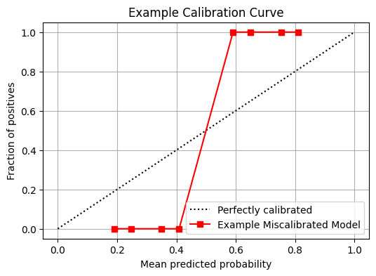
- The X-axis represents the model’s predicted probability, or its confidence (ranging from 0.0 to 1.0).
- The Y-axis represents the empirical frequency of the event, or the actual accuracy (the true fraction of positives).
To build this, you take thousands of predictions and group them into buckets or “bins” (for example, all predictions between 0.8 and 0.9). For each bin, you plot a single point: the average confidence on the X-axis versus the actual accuracy on the Y-axis.
The perfectly diagonal dashed line cutting through the center of the graph, where $y=x$. This is our gold standard. If a model is perfectly calibrated, every single point will fall exactly on this line. When the model says 80%, it is right 80% of the time.
How do we read deviations from this ideal?
- Points below the diagonal indicate overconfidence. The model is boasting a 0.9 probability, but the reality on the Y-axis is only 0.7.
- Points above the diagonal indicate underconfidence. The model timidly predicts 0.6, but it is actually correct 0.8 of the time.
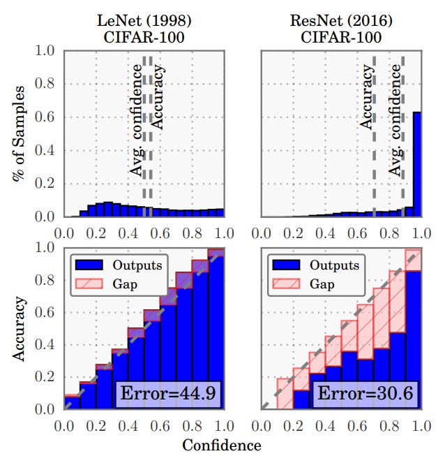
The Reality of Modern Neural Networks:
If you plot a modern, deep neural network (like a ResNet) on this diagram, you will rarely see a perfect diagonal. Instead, picture a curve that sags significantly below the diagonal line on the right side of the graph. This visual sag is the hallmark of modern deep learning: extreme overconfidence. The model frequently predicts probabilities near 0.99, but its actual accuracy in that bin might only be 0.85. Conversely, older, simpler models like Naive Bayes often form a curve that sits above the diagonal line, indicating they are systematically underconfident.
3. The Rigor: What “Calibrated” Means (and How to Measure It)
Now that we have established the intuition and the visual landscape, let us transition to the mathematical rigor. How do we formally define and measure this property?
3.1 The definition
For binary classification, a model produces a probability estimate $\hat{p}(x) \in [0,1]$. Perfect calibration means:
$$ \mathbb{P}(Y=1 \mid \hat{p}(X)=p) = p \quad \text{for all } p \in [0,1]. $$
In words: among all examples where the model says “$p$,” the event happens with frequency $p$.
A subtle but important point: conditioning on the event $\hat{p}(X)=p$ is mathematically clean, but for real-valued probabilities it can be a measure-zero event. That is why practical evaluation uses bins or smoothing: “among all predictions between 0.80 and 0.90, how often is the label positive?”
For multi-class classification with logits $\mathbf{z}(x) \in \mathbb{R}^K$ and predicted probabilities $\hat{\mathbf{p}}(x) \in [0,1]^K$, there are multiple sensible definitions in use:
- Class-wise calibration: for each class $k$, among all examples where $\hat{p}(Y=k\mid X)=p$, the event $Y=k$ occurs with frequency $p$.
- Top-label calibration: evaluate calibration for the model’s stated confidence in its predicted class, $\max_k \hat{p}(y=k\mid x)$.
When reading papers or dashboards, it is worth confirming which definition is being reported, because the same model can look well calibrated under one view and poorly calibrated under another.
3.2 Expected Calibration Error (ECE)
While the reliability diagram is excellent for visual inspection, we often need a single summary metric to quantify miscalibration—especially when comparing multiple models. This is where the Expected Calibration Error (ECE) comes in. It mathematically measures exactly what we visualized earlier: the gap between the model’s curve and the perfect diagonal.
To calculate ECE, partition predictions into $M$ bins (often equal-width; sometimes equal-mass). For each bin $B_m$, compute:
- the average predicted probability (confidence): $\text{conf}(B_m)$
- the empirical accuracy (fraction of positives): $\text{acc}(B_m)$
The ECE is the weighted average of the absolute differences between the accuracy and the confidence across all bins:
$$ \text{ECE} = \sum_{m=1}^{M} \frac{|B_m|}{n} \left|\text{acc}(B_m) – \text{conf}(B_m)\right| $$
where $n$ is the total number of samples and $|B_m|$ is the number of samples in bin $m$. A perfectly calibrated model has ECE $=0$.
Important nuance: ECE depends on binning (number of bins, equal-width versus equal-mass bins, and whether you bin top-label confidence or a class-conditional probability). For comparisons, keep the binning scheme fixed and consider reporting a complementary statistic such as the maximum calibration error (MCE), which replaces the weighted average with a maximum over bins.
If you only report a single ECE value, it is easy to miss problems concentrated in small regions (for example, very high confidence predictions that are rare but operationally important). In those cases, the reliability diagram itself and equal-mass bins are often more informative than a single aggregate number.
3.3 Brier score and negative log-likelihood
Another fundamental metric is the Brier Score, which measures the mean squared difference between the predicted probability $f_i$ and the actual outcome $o_i$. The Brier score for binary outcomes is:
$$ \text{BS} = \frac{1}{N} \sum_{i=1}^{N} (f_i – o_i)^2 $$
It is a proper scoring rule: it rewards well-calibrated probabilities and penalizes confident mistakes. Unlike ECE, it does not require binning. A lower score is better.
If you want a more “mechanistic” interpretation, the Brier score can be decomposed into terms that correspond to calibration and usefulness:
$$ \text{BS} = \text{reliability} – \text{resolution} + \text{uncertainty}. $$
Intuition:
- Reliability captures miscalibration (lower is better).
- Resolution captures how much predictions vary across groups (higher is better).
- Uncertainty is the intrinsic label noise/base-rate term for the dataset.
Another common proper scoring rule is negative log-likelihood (NLL) (log loss). For binary classification with predicted probability $f_i$:
$$ \text{NLL} = -\frac{1}{N}\sum_{i=1}^N \left[o_i\log(f_i) + (1-o_i)\log(1-f_i)\right]. $$
Temperature scaling is typically fit by minimizing NLL on a held-out calibration set.
4. Why Models Become Uncalibrated
Why do our most powerful, state-of-the-art models struggle so much with calibration? The answer becomes intuitive once we examine how we train them.
Look at the visual comparison below, contrasting older architectures (like LeNet) with modern ones (like ResNet). Notice how the modern network’s confidence distribution is heavily skewed toward 1.0, even when it is wrong.
Here are the primary culprits behind this phenomenon:
- The relentless push of cross-entropy. The standard cross-entropy loss function is never truly satisfied. Even after a model correctly classifies an image with 90% confidence, the loss function continues to penalize it, pushing the weights to achieve 99%, and then 99.9% confidence. It explicitly rewards extreme certainty, effectively training the model to be overconfident.
- Massive capacity meets limited data. Deep networks possess an enormous number of parameters. This high capacity allows them to fit the training distribution perfectly, carving out incredibly sharp decision boundaries that result in near-deterministic, highly confident scores.
- The side effects of modern regularization. Techniques like weight decay, batch normalization, and data augmentation are fantastic for improving accuracy, but they fundamentally alter the distribution of the model’s internal activations (logits). This often disconnects the raw logit scale from true probabilistic uncertainty.
- Dataset shift breaks calibration. A model calibrated on one hospital, region, or time period can become miscalibrated when the input distribution changes.
- Label noise and class imbalance distort probabilities. When labels are noisy or positives are rare, the model can learn probabilities that are systematically biased.
The key takeaway is that calibration is not only a model property; it is a property of a model and the data distribution on which it is evaluated.
There is also a practical “systems” reason this matters: calibration can look excellent on an i.i.d. test set and collapse in production if the deployment distribution changes. If a downstream policy uses confidence thresholds (triage, reject option, human-in-the-loop), even small miscalibration can translate into large operational surprises.
5. How to Calibrate Probabilities (Post-hoc)
Calibration is often applied as a post-processing step: train a predictive model as usual, then learn a mapping that converts its scores into better probabilities using a separate calibration dataset.
The most popular post-hoc methods are monotonic mappings. This is a crucial detail: monotonic functions preserve the relative order of the predictions. If the model ranked Patient A as higher risk than Patient B before calibration, Patient A will still be higher risk after calibration. The ranking (and thus metrics like AUC) stays exactly the same; we are simply reshaping the absolute confidence scale to reflect reality.
Three practical methods are:
- Platt scaling (logistic calibration). Fit a logistic regression model on the model’s scores (often logits or outputs of our uncalibrated classifier). This works well when the reliability diagram looks roughly S-shaped. It is a strong baseline and tends to behave well with smaller calibration sets.
- Isotonic regression. Fit a non-parametric, monotonically increasing step function. This is more flexible than Platt scaling but typically needs more calibration data to avoid overfitting. It can capture complex calibration curves but may produce a “staircase” mapping when the calibration split is small.
- Temperature scaling. This is the standard baseline for modern neural networks. It rescales logits by a single learned temperature $T>0$ before softmax: $$ \hat{p}(y=k\mid x;T)=\frac{\exp(z_k(x)/T)}{\sum_{j=1}^K \exp(z_j(x)/T)}. $$ For binary classification with logit $z(x)$, this becomes $\hat{p}(x)=\sigma(z(x)/T)$. Intuition: $T>1$ softens probabilities (reduces extreme confidence), and $T<1$ sharpens them. Temperature scaling typically preserves the predicted label (argmax), while improving probability quality.
If you need richer multi-class calibration than a single scalar temperature, there are extensions such as vector scaling and matrix scaling. In practice, they can overfit without sufficient calibration data, so the simplest method that meets the need is usually the best.
6. Implementation: A Leakage-Safe Calibration Workflow (scikit-learn)
Below is a practical example using isotonic regression as an explicit mapping on predicted probabilities. This avoids hidden cross-validation and makes the data separation obvious.
import numpy as np

from sklearn.datasets import make_classification
from sklearn.ensemble import RandomForestClassifier
from sklearn.isotonic import IsotonicRegression
from sklearn.metrics import brier_score_loss, log_loss
from sklearn.model_selection import train_test_split


def expected_calibration_error(y_true, y_prob, n_bins=15):
    """Simple ECE implementation for binary classification."""
    y_true = np.asarray(y_true)
    y_prob = np.asarray(y_prob)

    bin_edges = np.linspace(0.0, 1.0, n_bins + 1)
    bin_ids = np.digitize(y_prob, bin_edges[1:-1], right=False)

    ece = 0.0
    for b in range(n_bins):
        mask = bin_ids == b
        if not np.any(mask):
            continue
        bin_acc = np.mean(y_true[mask])
        bin_conf = np.mean(y_prob[mask])
        ece += (np.sum(mask) / y_true.size) * np.abs(bin_acc - bin_conf)
    return float(ece)


# 1. Synthetic dataset
X, y = make_classification(
    n_samples=10000,
    n_features=20,
    n_informative=10,
    n_redundant=5,
    weights=[0.7, 0.3],
    random_state=10,
)

# 2. Three-way split: train / calibration / test
X_train, X_temp, y_train, y_temp = train_test_split(
    X, y, test_size=0.4, random_state=42, stratify=y
)
X_cal, X_test, y_cal, y_test = train_test_split(
    X_temp, y_temp, test_size=0.5, random_state=42, stratify=y_temp
)

# 3. Train a base model (may be miscalibrated)
base = RandomForestClassifier(n_estimators=300, random_state=42)
base.fit(X_train, y_train)

prob_cal_uncal = base.predict_proba(X_cal)[:, 1]
prob_test_uncal = base.predict_proba(X_test)[:, 1]

# 4. Fit calibrator on the calibration split only
iso = IsotonicRegression(out_of_bounds="clip")
iso.fit(prob_cal_uncal, y_cal)

prob_test_cal = iso.predict(prob_test_uncal)

# 5. Evaluate on the test split
metrics = {
    "Brier": (
        brier_score_loss(y_test, prob_test_uncal),
        brier_score_loss(y_test, prob_test_cal),
    ),
    "NLL": (
        log_loss(y_test, np.c_[1 - prob_test_uncal, prob_test_uncal]),
        log_loss(y_test, np.c_[1 - prob_test_cal, prob_test_cal]),
    ),
    "ECE": (
        expected_calibration_error(y_test, prob_test_uncal),
        expected_calibration_error(y_test, prob_test_cal),
    ),
}

for name, (before, after) in metrics.items():
    print(f"{name}: uncalibrated={before:.4f} | calibrated={after:.4f}")

# Expected output:
#     Brier: uncalibrated=0.0496 | calibrated=0.0377
#     NLL: uncalibrated=0.1930 | calibrated=0.1674
#     ECE: uncalibrated=0.0860 | calibrated=0.0145

import matplotlib.pyplot as plt
from sklearn.calibration import calibration_curve

# Calculate calibration curve data for uncalibrated and calibrated predictions
fraction_of_positives_uncal, mean_predicted_value_uncal = calibration_curve(
    y_test, prob_test_uncal, n_bins=10
)
fraction_of_positives_cal, mean_predicted_value_cal = calibration_curve(
    y_test, prob_test_cal, n_bins=10
)

# Plot the calibration curves
plt.figure(figsize=(8, 6))
plt.plot([0, 1], [0, 1], "k:", label="Perfectly calibrated")
plt.plot(
    mean_predicted_value_uncal,
    fraction_of_positives_uncal,
    "s-",
    label="Uncalibrated Random Forest",
)
plt.plot(
    mean_predicted_value_cal,
    fraction_of_positives_cal,
    "o-",
    label="Calibrated Random Forest (Isotonic Regression)",
)

plt.xlabel("Mean predicted probability")
plt.ylabel("Fraction of positives")
plt.title("Calibration Curves")
plt.legend(loc="lower right")
plt.grid(True)
plt.show()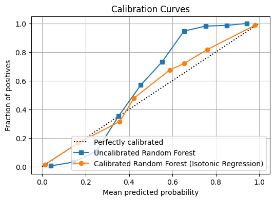
This example highlights the core rule: fit the base model on train, fit the calibrator on calibration, and report final metrics on test.
Note: the numeric values in the printed metrics can vary with random seeds, library versions, and dataset realizations. The qualitative pattern (proper scoring rules and ECE improving after calibration) is the point.
Two common pitfalls are (1) fitting the calibrator on the test set (which inflates reported performance) and (2) using too small a calibration set with isotonic regression (which can overfit and produce a “staircase” mapping).
7. Practical Tips and Best Practices
To ensure you are applying calibration correctly in your own engineering workflows, keep these core principles in mind:
- Always Use a Dedicated Hold-Out Set: Never calibrate your model on the same data you used to train it. If you do, the calibrator will simply memorize the model’s existing overconfidence, rendering the entire exercise useless. Always set aside a dedicated, unseen validation set specifically for fitting your calibrator.
- Choose the Right Method for Your Data:
- Use Platt Scaling (Logistic) when you have a smaller validation set (less than 1000 samples) to prevent overfitting.
- Use Isotonic Regression when you have a large validation set and you do not want to assume a specific shape for the calibration curve.
- Use Temperature Scaling if you are working with deep neural networks.
- Look Beyond Accuracy: Accuracy, Precision, and Recall do not tell you if your model is calibrated. You must calculate the Expected Calibration Error (ECE), the Brier Score, and visually inspect the Reliability Diagram to understand your model’s true confidence profile.
- Multi-Class Calibration: The methods discussed above are primarily for binary classification. For multi-class problems, Temperature Scaling is generally the most effective and easiest to implement, as it scales all logits uniformly without changing the predicted class labels.
- Treat ECE as a diagnostic, not a single truth. Report the binning scheme, and consider pairing ECE with a proper scoring rule (Brier or NLL).
- Re-calibrate after shifts. If the deployment distribution drifts, recalibration on fresh data is often cheaper than full retraining.

Happy is a seasoned ML professional with over 15 years of experience. His expertise spans various domains, including Computer Vision, Natural Language Processing (NLP), and Time Series analysis. He holds a PhD in Machine Learning from IIT Kharagpur and has furthered his research with postdoctoral experience at INRIA-Sophia Antipolis, France. Happy has a proven track record of delivering impactful ML solutions to clients.
Subscribe to our newsletter!