Think of a machine learning model as a high-performance engine prototype sitting on a pristine workbench. It might run beautifully in a controlled demonstration, but deploying it to production is like taking that engine out onto a real, unpredictable road. You will encounter messy fuel (data drift), changing weather conditions (traffic patterns), strict safety regulations (governance), and the inevitable need for maintenance schedules (retraining).
MLOps is the comprehensive set of practices that transforms these fragile model prototypes into reliable, observable, and reproducible software systems. It is a discipline that blends machine learning, software engineering, and DevOps across the entire lifecycle: data → training → validation → deployment → monitoring → iteration.
In this article, we will explore the practical steps, architecture patterns, and the common pitfalls that occur in the real world. We will start with the intuition behind why these systems fail, and then dive into the technical rigor required to keep them running smoothly.
1. Why MLOps Matters
In a production environment, building the model is rarely the most difficult part of the process. The true challenge lies in maintaining the correctness and reliability of the entire system over time.
1.1 Common Failure Modes
- Training–serving skew: The logic used to generate features differs between the offline training environment and the online inference environment.
- Silent data drift: The statistical distribution of the incoming data changes, causing model performance to decay without throwing explicit errors. Mathematically, we often distinguish between covariate shift (the input distribution $P(X)$ changes, but the relationship $P(Y|X)$ remains constant) and concept drift (the underlying relationship $P(Y|X)$ itself changes). Each requires distinct monitoring and retraining strategies.
- Label delay: Ground truth labels arrive late, meaning that monitoring systems must rely on proxy metrics to estimate performance.
- Reproducibility gaps: A team cannot recreate a specific model version because the data, code, or environment has changed and was not properly versioned.
- Operational fragility: The workloads are slow, prohibitively expensive, or unstable under high traffic load.
- Governance risk: There is an unknown data lineage, no formal approval process, and no audit trail for deployed models.
1.2 Outcomes MLOps Aims For
- Shorter iteration cycles: Teams can safely ship improvements and new features faster.
- Higher reliability: Deployments become predictable, resulting in fewer production incidents.
- Better model quality: Systematic evaluation, continuous monitoring, and automated retraining ensure the model remains accurate.
- Lower total cost: Compute and data storage costs become visible and controllable.
- Compliance readiness: Full traceability for data and models ensures the system is ready for audits.
2. MLOps in One Picture
Below is an end-to-end mental model of a typical MLOps system. Imagine a continuous, circular flow rather than a straight line.
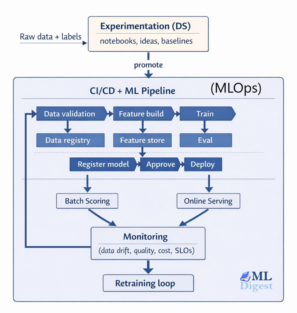
 Figure 1: The MLOps Lifecycle. Notice how production signals continuously feed back into the data collection and training phases.
The key idea here is that MLOps is not simply “deploy the model once and forget it.” It is a closed loop where production signals feed back into data collection, model training, and business decisions.
3. Core Concepts and Building Blocks
3.1 Version Everything (Data, Code, Environment)
To reproduce a model reliably, you need a complete “bill of materials.”
- Code version: The specific Git commit hash.
- Data version: An immutable snapshot of the dataset, or a query combined with a point-in-time snapshot.
- Environment: The exact Python version, a dependency lock file, and the container image digest.
- Configuration: All hyperparameters and pipeline parameters used during training.
Practical tip: Treat “a model” as a mathematical function $f(x; \theta, D, C, E)$ where $\theta$ represents the learned weights, $D$ is the data snapshot, $C$ is the configuration, and $E$ is the environment. If any single one of those variables is unknown, the model is fundamentally not reproducible.
3.2 Separate Experimentation from Production
Experimentation optimizes for creativity. Production optimizes for reliability.
The typical workflow separates the messy, exploratory phase from the automated, rigorous deployment phase.
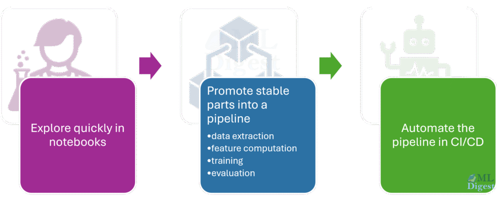
Figure 2: The transition from exploration (Jupyter notebooks, ad-hoc scripts) to deployment (versioned pipelines, CI/CD).
3.3 Define What “Good” Means (Metrics and Thresholds)
You must use a structured evaluation plan before a model ever sees production traffic:
- Offline metrics: Area Under the ROC Curve (AUC), F1-score, Root Mean Square Error (RMSE), calibration error, or ranking metrics.
- Slicing: Evaluate performance across specific regions, device types, user segments, or other sensitive cohorts to ensure equitable performance.
- Robustness: Test how the model handles missing values, noisy inputs, or out-of-range behavior.
- Fairness and safety: Implement checks depending on the specific domain and regulatory requirements.
- Business metrics: Measure conversion lift, cost per action, or latency impact.
Once these are defined, establish gates (automated checks that only allow deployment if specific thresholds are met).
3.4 Choose a Deployment Mode: Batch vs. Online
- Batch scoring: Run predictions on a scheduled basis and write the results to a database table.
- Pros: Simpler architecture, cheaper to run, easier to backfill historical data.
- Cons: Predictions are not available in real-time.
- Online serving: Provide synchronous inference via a REST or gRPC API.
- Pros: Real-time decision making.
- Cons: Harder to monitor, requires strict latency and Service Level Objective (SLO) management.
A hybrid approach is common: use online serving for immediate decisions and batch scoring for downstream analytics.
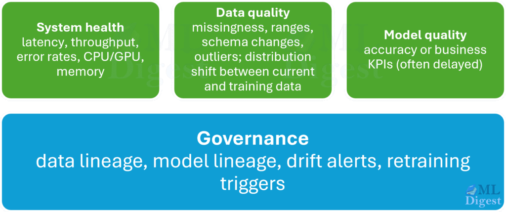
3.5 Monitoring is More Than “Model Accuracy”
Production monitoring usually consists of four distinct layers. Imagine a pyramid where infrastructure is the base and business metrics are the peak.
4. Implementation Steps (A Practical Roadmap)
This section outlines a “first production” path that most teams can adopt. You can implement these steps incrementally.
4.1 Step 0: Clarify the Product Contract
Before adopting any tools, write down the contract between the model and the business.
- Input contract: Define the schema, data types, units, and expectations for missing values.
- Output contract: Define what the prediction actually means, its expected range, and the decision thresholds.
- SLOs: Define acceptable latency, availability, and the cost per 1,000 predictions.
- Re-training triggers: Decide if retraining will be time-based, drift-based, or performance-based.
- Human-in-the-loop: Determine when a human operator needs to override the model’s predictions.
4.2 Step 1: Standardize Your Project Structure
Move away from a notebook-only approach to a minimal, standardized package layout. Use a structure similar to Cookiecutter Data Science or this GitHub repository or this blog post.
data/(or external tables): References and metadata.src/: Pipeline code (feature building, training, inference helpers).configs/: Configuration files for parameters.tests/: Unit tests for feature logic, preprocessing, and metrics.docs/: Design documents, runbooks, and monitoring plans.notebooks/: Exploration and analysis (strictly not for production code).scripts/: Entry points for training, evaluation, and inference.artifacts/: Model outputs, metrics, and logs. These should be reusable across training and inference to avoid skew.
Practical tip: If features are computed twice (once for training, once for serving), extract the feature code into a shared script or library to guarantee you avoid training-serving drift.
4.3 Step 2: Data Validation and Data Contracts
Add automated checks early in the pipeline. Start small with basic schema and constraint validation.
Here is a practical, runnable example of schema validation using the pandera library:
# pip install pandera pandas
import pandera as pa
import pandas as pd

# Define the expected schema for incoming data
class InputSchema(pa.DataFrameModel):
    user_id: pa.typing.Series[int] = pa.Field(gt=0)
    age: pa.typing.Series[int] = pa.Field(ge=0, le=120, nullable=True)
    country: pa.typing.Series[str]
    signup_days_ago: pa.typing.Series[int] = pa.Field(ge=0)

# Simulate some incoming data, including an invalid age (200)
df = pd.DataFrame(
    {
        "user_id": [1, 2, 3],
        "age": [34, None, 200],
        "country": ["US", "DE", "US"],
        "signup_days_ago": [10, 0, 5],
    }
)

# Ensure the age column uses pandas' nullable integer type
df["age"] = df["age"].astype(pd.Int64Dtype())

# Validate the dataframe against the schema
try:
    InputSchema.validate(df)
    print("Data validation passed.")
except pa.errors.SchemaErrors as e:
    print("Data validation failed!")
    print(e.failure_cases.head())
# Example output: SchemaError: Column 'age' failed element-wise validator number 1: less_than_or_equal_to(120) failure cases: 200How to use this in an MLOps context:
- Run this validation in the pipeline immediately before training.
- Run it during production inference to validate inputs (keeping careful watch on performance constraints).
- Store the validation results as artifacts for auditing.
4.4 Step 3: Features and Avoiding Training-Serving Skew
Options for feature management, ordered from simplest to most involved:
- Inline features: Compute features directly within the inference service (good for small, simple feature sets).
- Shared feature source code: Maintain one codebase that is imported and used by both the training pipeline and the serving service.
- Feature store: Use a centralized management system that guarantees point-in-time correctness.
Best practice: Strictly enforce point-in-time correctness for training data. If you accidentally use “future information” during training (known as label leakage), your offline metrics will look fantastic, but the model will fail in production.
4.5 Step 4: Training Pipeline with Tracked Experiments
Keep the training process as a deterministic mathematical function:
$$
\text{model} = \text{Train}(D_{\text{train}}, C) \quad \text{and} \quad \text{report} = \text{Evaluate}(\text{model}, D_{\text{valid}})
$$
You must track:
- The dataset snapshot ID.
- The code SHA (Git commit).
- The configuration parameters.
- The resulting metrics and plots.
- The artifacts (the serialized model file, preprocessing objects like scalers).
Here is an example skeleton of a robust training entrypoint:
from dataclasses import dataclass
from pathlib import Path
import json

@dataclass(frozen=True)
class TrainConfig:
    model_type: str
    random_seed: int
    output_dir: str

def train(cfg: TrainConfig) -> dict:
    # In a real scenario, replace this with actual training code (scikit-learn, PyTorch, etc.)
    # model = train_model(X_train, y_train, seed=cfg.random_seed)

    # Simulate evaluation metrics
    metrics = {
        "auc": 0.91,
        "calibration_error": 0.03,
    }

    # Ensure the output directory exists
    out = Path(cfg.output_dir)
    out.mkdir(parents=True, exist_ok=True)

    # Save the metrics to a JSON file for tracking
    (out / "metrics.json").write_text(json.dumps(metrics, indent=2))

    # Persist model artifacts here (e.g., joblib.dump, torch.save)
    # joblib.dump(model, out / "model.joblib")

    return metrics

if __name__ == "__main__":
    cfg = TrainConfig(model_type="logreg", random_seed=7, output_dir="artifacts/run_001")
print("Training completed. Metrics:", train(cfg))4.6 Step 5: Evaluation Gates (Promotion Rules)
Define strict rules that convert raw metrics into deployment decisions. For example:
- The AUC must improve by at least 0.5% over the current production baseline.
- The inference latency must be less than 50 milliseconds at the 95th percentile (p95).
- The performance must not regress on any critical data slice (e.g., performance on mobile users must remain stable).
- The model calibration must fall within a predefined tolerance band.
These rules become automated pipeline steps that either promote a model to a registry stage (e.g., “Staging”) or halt the pipeline and notify the owners.
4.7 Step 6: Model Registry and Approvals
A model registry acts as a central repository and provides:
- Storage for model artifacts.
- Metadata tracking (metrics, lineage).
- Lifecycle stages (Development → Staging → Production).
- Audit logs for compliance.
Even if you do not adopt a full registry tool initially, you should create a simple registry convention using your file system or cloud storage:
models/{model_name}/{run_id}/for storing artifacts.models/{model_name}/PRODUCTIONas a pointer file to the current active model.
However, adopting a dedicated tool like MLflow brings rigorous tracking. Here is a brief example of how you might log a model to a registry using MLflow:
import mlflow
import mlflow.sklearn
from sklearn.linear_model import LogisticRegression
from sklearn.datasets import make_classification

# Generate synthetic data and train a simple model
X_train, y_train = make_classification(n_samples=100, n_features=4, random_state=42)
model = LogisticRegression()
model.fit(X_train, y_train)

# Log the model to the MLflow registry
# Note: This requires an active MLflow tracking server
with mlflow.start_run() as run:
    mlflow.sklearn.log_model(
        sk_model=model,
        artifact_path="model",
        registered_model_name="user_conversion_model"
    )
print(f"Model registered successfully with run_id: {run.info.run_id}")4.8 Step 7: Deployment Strategies
Deployment is fundamentally a risk management problem. Choose a strategy that is appropriate for your domain’s risk tolerance.
- Shadow deployment: Run the new model in parallel with the old one. It processes real traffic but its predictions do not affect user decisions.
- Canary deployment: Route a small percentage (e.g., 5%) of live traffic to the new model to monitor its stability before a full rollout.
- Blue/green deployment: Maintain two identical production environments. Switch traffic entirely from the old environment (blue) to the new one (green).
- A/B testing: Compare two models in a controlled experiment to measure their impact on business metrics.
Online serving usually requires:
- Stable input schema validation.
- Strict feature parity across environments.
- Defined timeouts and fallback mechanisms (e.g., returning a default prediction if the model takes too long).
- Model warm-up procedures and concurrency testing.
4.9 Step 8: Monitoring and Alerting
Start with a monitoring plan that is highly actionable:
- What specific metrics will trigger an alert?
- Who is the designated person on call?
- What is the runbook (the step-by-step guide) to resolve the issue?
A common way to measure data drift is the Population Stability Index (PSI). It quantifies how much the distribution of a variable has shifted between two samples (e.g., training data vs. production data).
Mathematically, PSI is calculated by binning the data and comparing the proportions:
$$
\text{PSI} = \sum_{i=1}^{B} \left( \text{Actual}_i – \text{Expected}_i \right) \times \ln\left(\frac{\text{Actual}_i}{\text{Expected}_i}\right)
$$
Where $B$ is the number of bins, $\text{Actual}_i$ is the proportion of production data in bin $i$, and $\text{Expected}_i$ is the proportion of training data in bin $i$.
Here is a runnable implementation:
import numpy as np

def calculate_psi(expected: np.ndarray, actual: np.ndarray, bins: int = 10, eps: float = 1e-6) -> float:
    """
    Calculates the Population Stability Index (PSI) between two arrays.
    """
    # Define bin edges based on the quantiles of the expected (training) distribution
    quantiles = np.quantile(expected, np.linspace(0, 1, bins + 1))
    quantiles[0] -= eps
    quantiles[-1] += eps

    # Count how many samples fall into each bin
    exp_counts, _ = np.histogram(expected, bins=quantiles)
    act_counts, _ = np.histogram(actual, bins=quantiles)

    # Convert counts to proportions
    exp_props = exp_counts / max(exp_counts.sum(), 1)
    act_props = act_counts / max(act_counts.sum(), 1)

    # Clip to avoid division by zero or log(0)
    exp_props = np.clip(exp_props, eps, None)
    act_props = np.clip(act_props, eps, None)

    # Calculate the PSI formula
    psi_value = np.sum((act_props - exp_props) * np.log(act_props / exp_props))
    return float(psi_value)

# Example usage simulating a moderate drift
rng = np.random.default_rng(0)
train_feature = rng.normal(loc=0.0, scale=1.0, size=10_000)
prod_feature = rng.normal(loc=0.3, scale=1.2, size=10_000) # Shifted mean and variance

print(f"Calculated PSI: {calculate_psi(train_feature, prod_feature):.4f}")Interpretation heuristic (highly context-dependent):
- PSI < 0.1: Minor shift; no action required.
- 0.1 $\le$ PSI < 0.2: Moderate shift; investigate the cause.
- PSI $\ge$ 0.2: Large shift; likely requires retraining or immediate action.
4.10 Step 9: Continuous Improvement (Retraining Loop)
Common triggers for retraining a model:
- Time-based: Schedule weekly or monthly retraining pipelines.
- Drift-based: Trigger retraining automatically when data drift (like PSI) exceeds a defined threshold.
- Performance-based: Trigger retraining when online Key Performance Indicators (KPIs) regress.
Always implement safeguards for automated retraining:
- Strictly enforce evaluation gates before deploying the newly trained model.
- Maintain the capability to instantly rollback to the previous version.
- Keep the previous “champion” model and its exact data snapshot archived.
5. Scalability and Governance
As your machine learning system grows in complexity and usage, two new dimensions emerge: handling massive scale and ensuring strict compliance.
5.1 Designing for Scalability
When traffic spikes, your inference service must scale gracefully to maintain low latency.
- Horizontal Scaling: Deploy multiple replicas of your model behind a load balancer. Tools like Kubernetes (utilizing Horizontal Pod Autoscalers) or Ray Serve excel in this area.
- Compute Optimization: For deep learning models, serving on CPUs might be too slow, but keeping GPUs idle is prohibitively expensive. Techniques like dynamic batching (grouping incoming requests together before sending them to the GPU for processing) and model quantization (reducing the precision of weights, for example, from 32-bit floats to 8-bit integers) are essential for maximizing throughput and minimizing costs.
5.2 Enforcing Governance
Governance ensures that models are safe, ethical, and legally compliant.
- Model Cards: Inspired by the paper “Model Cards for Model Reporting” (Mitchell et al., 2019), every production model should have a standardized document detailing its intended use, the characteristics of its training data, and its performance across different demographic slices.
- Role-Based Access Control (RBAC): Not every engineer should have the permission to deploy a model directly to production. Implement strict approval workflows where a designated “Model Risk Officer” or lead data scientist must formally sign off on the deployment.
6. Practical Tips
6.1 Start Narrow, Then Generalize
Do not attempt to build a massive, generalized “ML platform” first. Pick one specific model, productionize it end-to-end, and then extract the reusable components for the next project.
6.2 Make Debugging Easy by Design
For every prediction made in production, try to log the following (while strictly adhering to privacy constraints):
- The exact model version.
- A summary or hashed representation of the input feature vector.
- The prediction output and a proxy for the model’s uncertainty.
- A unique request ID and user/session ID (if legally allowed).
- The latency of the request and the reason for any failure.
This comprehensive logging enables rapid root-cause analysis when a user inevitably reports that “the model behaved strangely.”
6.3 Treat Labeling as Part of the System
If ground truth labels arrive late or are expensive to acquire:
- Monitor proxy signals closely (e.g., input drift, changes in the prediction distribution).
- Improve the user interface to capture better implicit feedback channels.
- Prioritize labeling efforts on data points where the model is highly uncertain or where the downstream business impact is highest (a technique known as active learning).
6.4 Cost is a First-Class Metric
You must track:
- The compute cost per training run.
- The infrastructure cost per 1,000 inference requests.
- The storage costs for maintaining logs, data snapshots, and model artifacts.
Implement cost-aware practices:
- Use early stopping during training to save compute.
- Always evaluate cheaper, simpler baseline models before deploying massive deep neural networks.
- Utilize quantization or knowledge distillation for serving large models.
6.5 Reproducibility Recipe
At an absolute minimum, you must log:
git_shadata_snapshot_idconfig.jsonrequirements.txt(or a dependency lock file)- The exact training command line execution.
- The random seed used.
If possible, ensure all training runs are fully containerized using Docker to guarantee environment consistency.
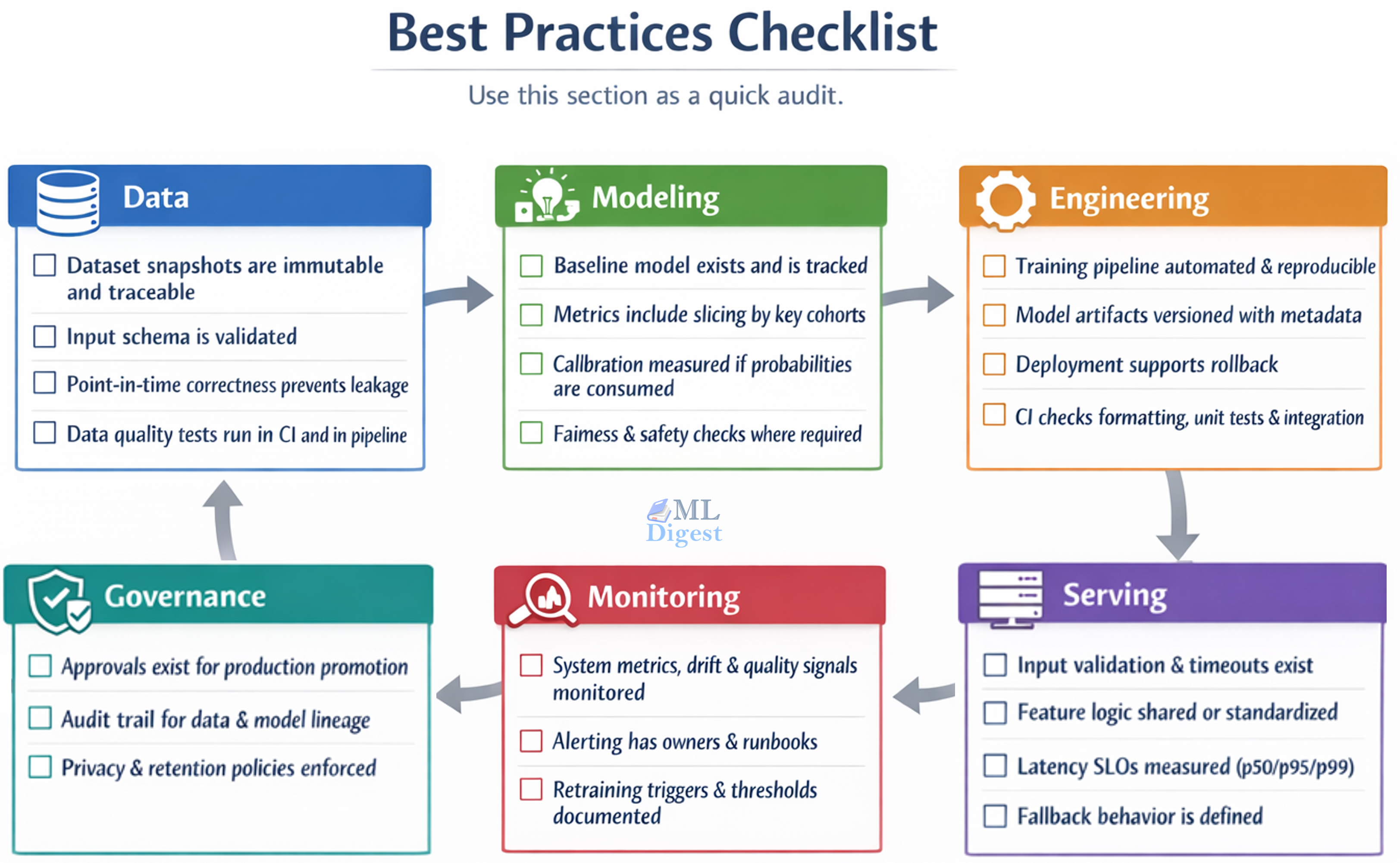
7. Best Practices Checklist
Imagine a radar chart tracking your MLOps maturity across several axes. As you implement better practices, your coverage expands outward.
- The Data Axis: The line extends outward as you implement immutable snapshots, strict schema validation, and point-in-time correctness to prevent data leakage.
- The Modeling Axis: The line pushes outward when you track baseline models, slice metrics by key cohorts, and enforce fairness and calibration checks.
- The Engineering Axis: Maturity grows here through automated, reproducible training pipelines, versioned model artifacts, and rigorous Continuous Integration (CI) checks.
- The Serving Axis: This axis expands as you add strict input validation, shared feature logic between training and serving, and defined fallback behaviors for when the model fails.
- The Monitoring Axis: The line reaches the outer edge when you actively monitor system metrics and data drift, maintain alerting runbooks, and document automated retraining triggers.
- The Governance Axis: The final axis extends outward with formal production approvals, comprehensive audit trails for data lineage, and strict privacy policy enforcement.
Tooling Map
You can implement MLOps using many different combinations of tools. Below is a practical map of tool categories to help you choose what fits your existing stack.
%%{init: {'theme': 'base', 'themeVariables': {
    'fontSize': '24px',
    'fontFamily': 'Arial',
    'primaryTextColor': '#000000'
}}}%%

flowchart TD
    subgraph "MLOps Tooling Landscape"
        direction LR
        Data["<b>Data & Features</b><br/>DVC, Delta Lake,<br/>Feast, Tecton"]
        Orch["<b>Orchestration</b><br/>Airflow, Prefect,<br/>Dagster, Kubeflow"]
        Track["<b>Tracking & Registry</b><br/>MLflow, W&B,<br/>Comet"]
        Test["<b>Testing & Validation</b><br/>Great Expectations,<br/>Pandera, pytest"]
        Serve["<b>Serving</b><br/>FastAPI, Flask,<br/>BentoML, KServe"]
        Mon["<b>Monitoring</b><br/>Prometheus, Grafana,<br/>EvidentlyAI"]

        Data --> Orch
        Orch --> Track
        Track --> Test
        Test --> Serve
        Serve --> Mon
        Mon -.->|"Feedback"| Data
    end
A Simple Operating Model
MLOps is collaborative by design. Clear ownership prevents the dangerous scenario where “nobody owns production.”
- Data scientists: Responsible for problem framing, modeling, evaluation design, and error analysis.
- ML engineers: Responsible for building pipelines, ensuring feature parity, managing serving infrastructure, and optimizing performance and reliability.
- Platform/DevOps engineers: Responsible for underlying infrastructure, CI/CD pipelines, security, scaling, and cost controls.
- Product and domain experts: Responsible for defining success metrics, establishing feedback loops, and setting business constraints.
Practical tip: Assign a single, named “model owner” for every model in production, even if many people contribute to its development.
Summary
MLOps turns the art of machine learning into a disciplined, reliable production practice. The core pattern is a continuous, closed loop:
- Validate and version your data.
- Train and evaluate models with strict reproducibility.
- Promote models using automated gates and formal approvals.
- Deploy using safe, controlled rollout strategies.
- Monitor system health, data drift, and business impact continuously.
- Retrain and improve the system with established guardrails.

Silpa brings 5 years of experience in working on diverse ML projects, specializing in designing end-to-end ML systems tailored for real-time applications. Her background in statistics (Bachelor of Technology) provides a strong foundation for her work in the field. Silpa is also the driving force behind the development of the content you find on this site.

Happy is a seasoned ML professional with over 15 years of experience. His expertise spans various domains, including Computer Vision, Natural Language Processing (NLP), and Time Series analysis. He holds a PhD in Machine Learning from IIT Kharagpur and has furthered his research with postdoctoral experience at INRIA-Sophia Antipolis, France. Happy has a proven track record of delivering impactful ML solutions to clients.
Subscribe to our newsletter!