Understanding Diffusion Models: How AI Generates Images from Noise

Imagine standing in an art gallery, looking at a detailed photograph of a landscape. Now imagine a thick fog slowly rolling in. At first, edges soften. Then fine details disappear. Eventually, everything becomes a flat wall of static.

Now ask a precise question: Can the fog be reversed? More formally, can one start from (almost) pure noise and recover a realistic image by applying a sequence of small, local corrections?

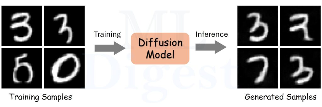
For a human, this reconstruction seems impossible. However, this is exactly what diffusion models are trained to approximate. By learning to reverse a carefully designed destruction process, they gain the ability to create new, realistic samples from scratch.

We will explore the technology that powers DALL-E, Stable Diffusion, and Midjourney. We will start with the intuition, dive into the rigorous mathematics, and finally build the core components in Python.

1. The Intuition: Destruction and Restoration

To understand diffusion models, separate two processes that run in opposite directions over a sequence of timesteps:

the Forward Process (Destruction), which gradually adds noise, and
the Reverse Process (Creation), which attempts to remove that noise step by step.

The figure below illustrates this idea: a real image is progressively corrupted by noise (forward direction), then iteratively denoised back toward a clean sample (reverse direction).

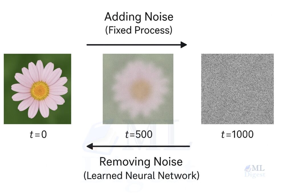
The Forward Process (The “Fog”)

Think of the forward process as repeatedly adding small amounts of Gaussian noise.

Step 0: You have a clear image of a flower.
Step 1: You add a tiny bit of Gaussian noise (static). The flower is still visible, just grainy.
Step 100: You have added more noise. The flower is barely recognizable.
Step 1000: The image is pure random noise. No trace of the flower remains.

This process is easy to implement. No neural network is needed to destroy an image; a fixed formula injects Gaussian noise at each step. The forward process is therefore entirely known and controllable (and is chosen by the practitioner).

The Reverse Process (The “Un-Fogging”)

The reverse process is where learning enters. At each timestep, the model examines a noisy image and answers a specific question:

What noise was added at this step to produce what I see now?

If the model can predict the noise accurately, you can subtract this estimate to obtain a slightly clearer image. Repeating this “predict noise → subtract noise” step across many timesteps walks you gradually from pure static back to a crisp, high-resolution image.

Conceptually, the model is not directly asked to “generate a cat” or “restore the mountains.” It is asked to become very good at small denoising steps. Composing thousands of such steps yields coherent, high-quality images.

2. Why Diffusion Models? Why They Matter

Before diffusion models became a dominant approach for image generation, practitioners primarily used GANs (Generative Adversarial Networks) and VAEs (Variational Autoencoders). Diffusion models rose to prominence for several reasons:

Stability: Diffusion training optimizes a single, well‑defined loss. This avoids the unstable adversarial dynamics of GANs—two networks fighting each other—which commonly cause mode collapse or oscillation. Compared with VAEs, which optimize a variational lower bound and often yield over‑smoothed or blurry outputs, diffusion training behaves more like supervised regression across noise levels, making convergence and debugging more predictable.
High sample quality and diversity:
Empirically, diffusion models produce very high-fidelity samples while capturing rich, multimodal structure in the data. They tend to generate a broader variety of realistic outputs instead of collapsing to a narrow subset of possibilities. This is particularly valuable for complex, real-world image distributions.
Conceptually simple objective:
The core prediction task is straightforward: given a noisy image and a timestep, predict the Gaussian noise that was added. This yields a simple Mean Squared Error loss that is easy to implement, stable to optimize, and scales well to large datasets and models.

Their practical impact was also cemented by two innovations that made diffusion models usable at scale:

Cross-attention (text-to-image): Diffusion models proved to be much better at “listening” to text prompts. By using attention mechanisms (as popularized by Transformer models), systems such as Stable Diffusion and DALL-E can map words to specific denoising steps far more accurately than GAN-based approaches typically could.
The latent diffusion breakthrough: Early diffusion models were often too slow because they operated directly on pixels. Researchers moved the diffusion process into a latent space by first compressing images with an autoencoder. The model then performs the iterative denoising in this smaller, structured representation, which dramatically reduces compute and makes high-quality generation feasible on consumer GPUs.

Feature	GAN (Adversarial)	VAE (Probabilistic)	Diffusion (Iterative)
Training Goal	Fool a “Critic” network	Reconstruct compressed data	Predict and remove noise
Training Stability	Very Unstable (oscillates, adversarial collapse)	Highly Stable and well-behaved	Extremely stable, simple supervised objective
Image Quality	Very sharp but inconsistent	Consistent, but blurry	Sharp, high-fidelity, and perceptually realistic
Diversity	Poor; prone to mode collapse	Good coverage of data distribution	Excellent coverage with high diversity
Conditioning	Fragile and difficult to control	Limited and low-fidelity	Strong, flexible, and robust across modalities
Generation Speed	Fast (Single pass)	Fast (Single pass)	Slow (Multi-step)
Scaling	Degrades and destabilizes at scale	Moderate scaling, bottlenecked by latent	Scales smoothly with data, compute, and model size
Engineering simplicity	Complex and fragile to tune	Relatively simple but limited	Simple, predictable, and easy to debug

From an engineering perspective, the combination of stability, sample quality, and conceptual simplicity made diffusion models an attractive successor to GANs for many applications.

Why Diffusion Models Beat GANs?

Why Diffusion Models Beat GANs: Stability, Coverage, and Control

For years, GANs were the industry standard for high-quality generation, but they suffer from two deep, structural problems that diffusion models fundamentally solved.

1. Mode Collapse vs. Distribution Coverage
GANs are prone to mode collapse: if the generator discovers a narrow set of outputs that reliably fool the discriminator (e.g., one perfect-looking cat), it may stop exploring the rest of the data distribution altogether. As a result, GANs often produce sharp images but miss entire modes—different object categories, poses, or styles never appear.

Diffusion models, by contrast, are trained with a likelihood-based objective (typically noise prediction or score matching). This objective explicitly encourages the model to explain all training data, not just a subset that wins an adversarial game. The result is far better coverage of the full data distribution: diverse objects, scenes, and styles all appear naturally.

2. Training Stability: The Biggest Practical Win
Training a GAN is a fragile min–max optimization problem. The generator and discriminator must remain perfectly balanced; if either becomes too strong, training oscillates, collapses, or diverges entirely. Small changes in learning rate, architecture, or batch size can break training, making GANs notoriously hard to scale and debug.

Diffusion models remove the adversary altogether. They are trained with a simple supervised loss (often mean-squared error on predicted noise), which is typically well-behaved in practice. There is no generator–discriminator arms race and far fewer failure modes related to balancing two networks, which improves scalability and debuggability.

3. Conditioning and Scalability
GANs also struggled with conditional generation. Conditioning on text, audio, or complex structure often required fragile architectural tricks and still produced unstable results. Diffusion models incorporate conditioning naturally at every denoising step, making text-to-image, image editing, audio, video, and even 3D generation straightforward and robust.

Finally, diffusion models tend to scale smoothly with more data, larger models, and more compute, aligning well with modern GPU/TPU training pipelines. GANs, in contrast, often become harder to keep stable as scale increases.

Why Diffusion Models Beat VAEs?

Why Diffusion Models Beat VAEs: Sharpness Through Iterative Refinement

VAEs were always praised for their theoretical grounding and training stability, but they suffered from a persistent and critical weakness: blurry outputs. Diffusion models retain stability while eliminating this problem.

1. The Lossy Latent Bottleneck Problem
VAEs compress images into a small latent representation and then decode them back into pixel space. This compression is inherently lossy. Fine-grained details—skin texture, hair strands, leaf structure—are often discarded because the latent bottleneck cannot represent them precisely. When decoded, the model produces averaged reconstructions, which manifest visually as blur.

Diffusion models avoid the single-shot reconstruction bottleneck. They refine samples iteratively in data space (or in a lightly compressed latent), so fine details can be introduced gradually rather than being forced through one latent code.

2. Iterative Denoising = Precision
Instead of generating an image in one shot, diffusion models start from pure noise and refine it through hundreds or thousands of tiny steps. Early steps focus on global structure—layout, composition, and object placement—while later steps add increasingly fine details.

This iterative refinement allows diffusion models to “sculpt” images with extreme precision. By the final steps, the model is free to focus entirely on micro-textures and sharp edges, producing results that are both globally coherent and richly detailed—something VAEs consistently struggled to achieve.

3. Best of Both Worlds: Sharp and Complete
VAEs optimize likelihood and therefore cover the data distribution well, but they sacrifice sharpness. GANs produce sharp images but often miss modes. Diffusion models achieve both:

Complete coverage of the data distribution
High perceptual fidelity
Excellent global structure and fine detail

They also scale predictably with model size, dataset size, and training time, and integrate seamlessly with modern architectures like U-Nets, Transformers, and attention mechanisms. In short, diffusion models combine the stability of VAEs with image quality that surpasses GANs—making them the dominant paradigm for modern generative modeling.

3. The Mathematics: From Intuition to Rigor

In practice, most modern diffusion systems build on Denoising Diffusion Probabilistic Models (DDPMs). DDPM is a disciplined version of the fog story: it defines a known forward corruption process that turns data into nearly Gaussian noise, then trains a neural network to approximately reverse that process one small step at a time.

DDPM provides three pieces of structure:

A tractable forward process $q$ that you can sample from and analyze. This process is fixed and does not need learning.
A learned reverse process $p_\theta$ that is expressive enough to model complex image distributions. This is the learned part.
A simple training objective (typically an MSE on predicted noise) that behaves like supervised learning across many noise levels.

The Forward Process $q$

Start with real data $x_{0}$ (for example, an image).
Gradually add Gaussian noise over many steps:
$$x_{0} \rightarrow x_{1} \rightarrow x_{2} \rightarrow \dots \rightarrow x_{T}$$
After enough steps, the data becomes pure noise.

Let us now formalize the process. Treat the sequence of noisy images as a Markov chain of $T$ steps. “Markov” means that $x_t$ depends only on $x_{t-1}$ (not the full history) given the noise injected at step $t$.

Define a schedule of variances $\beta_t$ that controls how much noise is added at each step. Given $x_{t-1}$, the next state $x_t$ is Gaussian:

$$ q(x_t | x_{t-1}) = \mathcal{N}(x_t; \sqrt{1 – \beta_t} x_{t-1}, \beta_t \mathbf{I}) $$

This expression encodes the idea: scale the previous image by $\sqrt{1-\beta_t}$ and add Gaussian noise with variance $\beta_t$. Larger $\beta_t$ means a more aggressive corruption step.

The above equation is equivalent to:

$$x_{t} = \sqrt{1 – \beta_{t}} x_{t – 1} + \sqrt{\beta_{t}} \epsilon , \qquad \epsilon \sim \mathcal{N} \left(\right. 0 , I_{d} \left.\right) .$$

Here $\epsilon$ is standard Gaussian noise. The dimension $d$ is the number of scalar values in the representation (for pixel space, the number of pixels times channels), and $x_t, x_{t-1} \in \mathbb{R}^d$. For a $64 \times 64$ RGB image, $d = 64 \times 64 \times 3 = 12{,}288$.

A powerful property of this process is that it is not necessary to simulate all intermediate steps $1, \dots, t – 1$ to get to step $t$. One can jump directly to any timestep $t$ using a closed-form expression. Let $\alpha_t = 1 – \beta_t$ and $\bar{\alpha}_t = \prod_{i=1}^t \alpha_i$.

$$ \begin{align} x_{t} &= \sqrt{\alpha_t} x_{t – 1} + \sqrt{1 – \alpha_t} \epsilon \\
&= \sqrt{\alpha_t} \left(\sqrt{\alpha_{t-1}} x_{t – 2} + \sqrt{1 – \alpha_{t-1}} \epsilon\right) + \sqrt{1 – \alpha_t} \epsilon \\
&= \sqrt{\alpha_t \alpha_{t-1}} x_{t – 2} + \sqrt{1 – \alpha_t \alpha_{t-1}} \epsilon \\
&= … \\
&= \sqrt{\bar{\alpha}_t} x_0 + \sqrt{1 – \bar{\alpha}_t} \epsilon
\end{align} $$

Thus, the distribution of $x_t$ given the original image $x_0$ is also Gaussian (see Lilian Weng’s blog post or this survey paper for detailed derivations):
$$ q(x_t | x_0) = \mathcal{N}(x_t; \sqrt{\bar{\alpha}_t} x_0, (1 – \bar{\alpha}_t)\mathbf{I}) $$

By multiplying the $\alpha_i$ terms across timesteps, we can compute how much of the original image $x_0$ survives at any later timestep $t$. The scalar $\sqrt{\bar{\alpha}_t}$ measures the remaining signal, and $\sqrt{1 – \bar{\alpha}_t}$ measures the cumulative noise.

This allows you to sample $x_t$ directly from the original image $x_0$ in a single step:
$$ x_t = \sqrt{\bar{\alpha}_t} x_0 + \sqrt{1 – \bar{\alpha}_t} \epsilon $$
where $\epsilon \sim \mathcal{N}(0, \mathbf{I})$ is pure noise.

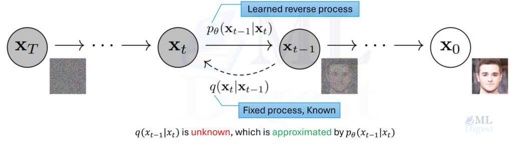
The Reverse Process $p_\theta$

The model learns how to reverse the noise process:
$$x_{T} \rightarrow x_{T – 1} \rightarrow \dots \rightarrow x_{0}$$
At each step, a neural network predicts the noise and removes it.

The mathematically ideal reverse distribution would be $q(x_{t-1} | x_t)$: given a noisy image $x_t$, what is the distribution over slightly less noisy states $x_{t-1}$ that could have produced it? Computing this exactly requires knowledge of the true data distribution, which is intractable.

Instead, we approximate it using a neural network with parameters $\theta$:
$$ p_\theta(x_{t-1} | x_t) = \mathcal{N}(x_{t-1}; \mu_\theta(x_t, t), \Sigma_\theta(x_t, t)) $$
where $\theta$ denotes model parameters, and the mean $\mu_\theta(x_t, t)$ and variance $\Sigma_\theta(x_t, t)$ are parameterized by deep neural network.

Read this as: “Given the current noisy image $x_t$ and the timestep $t$, the model proposes a distribution over slightly less noisy images $x_{t-1}$.” In practice, many implementations usually fix the variance $\Sigma_\theta$ to a known function of $t$ and only train the network to predict the mean $\mu_\theta$. This keeps the parameterization simple while still yielding good results.

The Objective Function

Under the DDPM formulation, predicting the mean $\mu_\theta(x_t,t)$ can be written in terms of predicting the noise $\epsilon_\theta(x_t,t)$ that was added. This turns learning into a regression problem with a clear target.

The loss function simplifies to a Mean Squared Error (MSE) between the actual noise added ($\epsilon$) and the predicted noise ($\epsilon_\theta$) (as discussed in this paper):

$$
\begin{align} L_{simple} &= \mathbb{E}_{t, x_0, \epsilon} \left[\lVert \epsilon – \epsilon_\theta(x_t,t) \rVert^2\right]\\
&= \mathbb{E}_{t, x_0, \epsilon} [ \lVert \epsilon – \epsilon_\theta(\sqrt{\bar{\alpha}_t} x_0 + \sqrt{1 – \bar{\alpha}_t} \epsilon, t) \rVert^2 ] \end{align}
$$

This objective says: across many different noise levels $t$ and many different images $x_0$, teach the model to reconstruct the exact noise sample that corrupted $x_0$ into $x_t$. If the model succeeds at this task for all levels of noise, then at sampling time we can run the process backward: starting from pure noise, repeatedly predict and subtract the noise to reveal synthetic images that follow the training distribution.

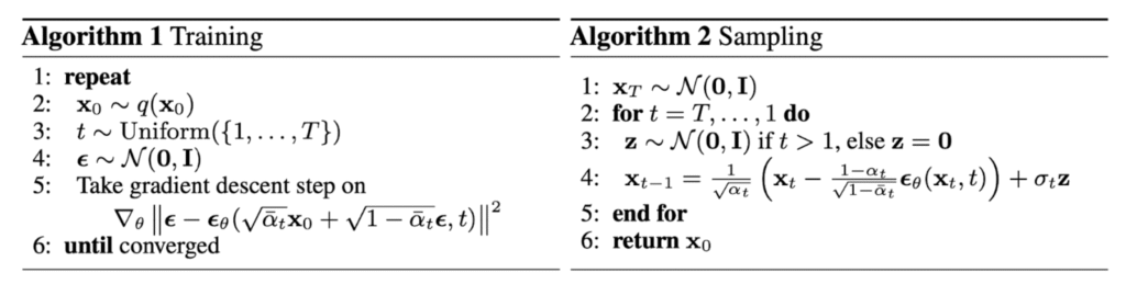
You can read this as the following sampling-and-training procedure:

Pick a random image $x_0$ from the dataset.
Pick a random timestep $t$.
Generate random noise $\epsilon$.
Corrupt the image to create $x_t$ using the closed-form forward process.
Ask the neural network: given $x_t$ and $t$, predict the noise $\epsilon$.
Compute the error and update the network parameters.

In words: the model is trained to be a noise predictor at many noise levels. The forward process is analytically defined and used only to generate training pairs $(x_t, \epsilon)$, while the reverse process is learned and parameterized by the neural network.

This perspective explains the practical appeal: diffusion training looks like supervised learning across a continuum of noise levels.

DDPM-algo — (The training and sampling algorithms in DDPM (Image source: paper)

Key Equations (Quick Reference)

If you remember only three lines, remember these:

One forward step:
$$q(x_t \mid x_{t-1}) = \mathcal{N}\left(x_t; \sqrt{1-\beta_t}\,x_{t-1},\;\beta_t\mathbf{I}\right)$$
Jump to any timestep:
$$x_t = \sqrt{\bar{\alpha}_t}\,x_0 + \sqrt{1-\bar{\alpha}_t}\,\epsilon, \qquad \epsilon \sim \mathcal{N}(0,\mathbf{I})$$
Training signal (noise prediction):
$$L_{simple} = \mathbb{E}\left[\lVert \epsilon – \epsilon_\theta(x_t,t) \rVert^2\right]$$

diffusion-model-progressive-generation-unconditional — (Unconditional progressive generation from paper)

4. Implementation: Building the Core

The following implementation mirrors the mathematical story above in a minimal PyTorch setup. The goal is not to achieve state-of-the-art performance, but to make each component of the diffusion process concrete:

a schedule that defines how noise is added,
a function that samples noisy images at arbitrary timesteps,
a U-Net-style neural network that predicts noise, and
a training step that ties all of these together.

diffusion-model-implementation — (Example outputs from the implementation below after training on a few samples of digit dataset for several thousand steps.)

Let us now implement the forward diffusion process and the training loop structure in Python using PyTorch.

Python

import torch
import torch.nn as nn
import torch.nn.functional as F
import numpy as np

### Step 1: The Noise Schedule
# We need to define $\beta_t$ and calculate $\bar{\alpha}_t$.

class DiffusionSchedule:
    def __init__(self, timesteps=1000, beta_start=1e-4, beta_end=0.02, device="cpu"):
        self.timesteps = timesteps
        self.device = device

        # Define linear beta schedule
        self.betas = torch.linspace(beta_start, beta_end, timesteps).to(device)

        # Pre-calculate alpha terms
        self.alphas = 1.0 - self.betas
        # This is alpha_bar_t = prod_{s=1}^t alpha_s
        self.alphas_cumprod = torch.cumprod(self.alphas, axis=0)

    def forward_diffusion(self, x_0, t):
        """Takes an image x_0 and a timestep t, and returns x_t and the noise added.

        Args:
            x_0: Clean images, shape [B, C, H, W].
            t: Timesteps, shape [B], each in [0, timesteps).
        Returns:
            x_t: Noisy images at timestep t.
            epsilon: The Gaussian noise that was added.
        """
        # Ensure tensors are on the same device as the input
        device = x_0.device

        # Extract alpha_bar for the specific timesteps t
        sqrt_alphas_cumprod = torch.sqrt(self.alphas_cumprod[t]).to(device)
        sqrt_one_minus_alphas_cumprod = torch.sqrt(1.0 - self.alphas_cumprod[t]).to(device)

        # Reshape for broadcasting (assuming x_0 is [Batch, Channels, Height, Width])
        sqrt_alphas_cumprod = sqrt_alphas_cumprod.view(-1, 1, 1, 1)
        sqrt_one_minus_alphas_cumprod = sqrt_one_minus_alphas_cumprod.view(-1, 1, 1, 1)

        # Generate random noise
        epsilon = torch.randn_like(x_0).to(device)

        # Apply the formula: x_t = sqrt(alpha_bar) * x_0 + sqrt(1 - alpha_bar) * epsilon
        x_t = sqrt_alphas_cumprod * x_0 + sqrt_one_minus_alphas_cumprod * epsilon

    return x_t, epsilon

# The `DiffusionSchedule` class encapsulates the **forward process** $q(x_t | x_0)$. It stores the per-timestep noise variances $\beta_t$, the corresponding signal retention factors $\alpha_t$, and their cumulative product $\bar{\alpha}_t$. The method `forward_diffusion` implements the closed-form sampling equation

# $$ x_t = \sqrt{\bar{\alpha}_t} x_0 + \sqrt{1 - \bar{\alpha}_t} \epsilon, $$

# returning both the noisy image $x_t$ and the specific noise sample $\epsilon$ that was used, which becomes the supervision signal for the neural network.

### Step 2: The Neural Network (The Noise Predictor)

## A minimal U‑Net‑style noise predictor

# The standard architecture used in diffusion models is a **U-Net**: an encoder–decoder with skip connections that preserves spatial information. It takes the noisy image $x_t$ and the timestep $t$ as input, and outputs a tensor of the same shape representing the predicted noise.

# Below is a **minimal, simplified** U‑Net‑like model that is good enough for toy datasets (e.g., $32\times 32$ or $64\times 64$ images). The goal is readability, not state‑of‑the‑art performance.

class TimeEmbedding(nn.Module):
    """Sinusoidal timestep embedding followed by an MLP."""

    def __init__(self, dim: int):
        super().__init__()
        self.dim = dim
        self.fc1 = nn.Linear(dim, dim)
        self.fc2 = nn.Linear(dim, dim)

    def forward(self, t):
        # t: [B] (integer timesteps)
        half = self.dim // 2
        device = t.device
        # positional encodings in log space
        freqs = torch.exp(
            -torch.linspace(0, np.log(10000), half, device=device)
        )  # [half]
        args = t[:, None].float() * freqs[None]  # [B, half]
        emb = torch.cat([torch.sin(args), torch.cos(args)], dim=-1)  # [B, dim]
        emb = F.silu(self.fc1(emb))
        emb = self.fc2(emb)
        return emb  # [B, dim]


class ResidualBlock(nn.Module):
    def __init__(self, in_channels, out_channels, time_dim):
        super().__init__()
        self.conv1 = nn.Conv2d(in_channels, out_channels, 3, padding=1)
        self.conv2 = nn.Conv2d(out_channels, out_channels, 3, padding=1)
        self.time_proj = nn.Linear(time_dim, out_channels)
        self.skip = (
            nn.Conv2d(in_channels, out_channels, 1)
            if in_channels != out_channels
            else nn.Identity()
        )

    def forward(self, x, t_emb):
        # x: [B, C, H, W], t_emb: [B, time_dim]
        h = self.conv1(x)
        # Add time embedding as bias
        h = h + self.time_proj(t_emb)[:, :, None, None]
        h = F.silu(h)
        h = self.conv2(h)
        return F.silu(h + self.skip(x))


class SimpleUNet(nn.Module):
    def __init__(self, in_channels=3, base_channels=64, time_dim=128):
        super().__init__()
        self.time_embed = TimeEmbedding(time_dim)

        # Encoder
        self.down1 = ResidualBlock(in_channels, base_channels, time_dim)
        self.down2 = ResidualBlock(base_channels, base_channels * 2, time_dim)
        self.pool = nn.MaxPool2d(2)

        # Bottleneck
        self.bottleneck = ResidualBlock(base_channels * 2, base_channels * 2, time_dim)

        # Decoder
        self.up = nn.Upsample(scale_factor=2, mode="nearest")
        self.up1 = ResidualBlock(base_channels * 2 + base_channels, base_channels, time_dim)
        self.out_conv = nn.Conv2d(base_channels, in_channels, 3, padding=1)

    def forward(self, x, t):
        # x: [B, C, H, W]
        # t: [B]
        t_emb = self.time_embed(t)

        # Encoder
        h1 = self.down1(x, t_emb)      # [B, base, H, W]
        h2 = self.down2(self.pool(h1), t_emb)  # [B, 2*base, H/2, W/2]

        # Bottleneck
        hb = self.bottleneck(h2, t_emb)

        # Decoder with skip connection from h1
        up = self.up(hb)  # [B, 2*base, H, W]
        up = torch.cat([up, h1], dim=1)
        hu = self.up1(up, t_emb)

        # Final prediction: same shape as input image
    return self.out_conv(hu)

# The `SimpleUNet` model plays the role of $\epsilon_\theta(x_t, t)$ in the equations. It receives the noisy image $x_t$ (a tensor of shape `[B, C, H, W]`) and the scalar timestep $t$ (one per image in the batch), and outputs a tensor of the same shape as $x_t$ that represents the **predicted noise**. The U-Net architecture allows the model to combine local texture information with global structure while preserving spatial resolution, which is important for high-quality denoising.


### 4.4 Step 3: The Training Loop

# Here is how to train the model to become an expert denoiser.

def train_one_step(model, optimizer, x_0, diffusion_schedule, device):
    optimizer.zero_grad()

    # 1. Sample random timesteps for each image in the batch
    batch_size = x_0.shape[0]
    t = torch.randint(0, diffusion_schedule.timesteps, (batch_size,), device=device).long()

    # 2. Create noisy images x_t
    x_t, noise_added = diffusion_schedule.forward_diffusion(x_0, t)

    # 3. Predict the noise using the model
    noise_predicted = model(x_t, t)

    # 4. Calculate Loss (MSE between actual noise and predicted noise)
    loss = F.mse_loss(noise_predicted, noise_added)

    # 5. Backpropagation
    loss.backward()
    optimizer.step()

    return loss.item()

import torch
import torch.nn as nn
import torch.nn.functional as F
import numpy as np

### Step 1: The Noise Schedule
# We need to define $\beta_t$ and calculate $\bar{\alpha}_t$.

class DiffusionSchedule:
    def __init__(self, timesteps=1000, beta_start=1e-4, beta_end=0.02, device="cpu"):
        self.timesteps = timesteps
        self.device = device

        # Define linear beta schedule
        self.betas = torch.linspace(beta_start, beta_end, timesteps).to(device)

        # Pre-calculate alpha terms
        self.alphas = 1.0 - self.betas
        # This is alpha_bar_t = prod_{s=1}^t alpha_s
        self.alphas_cumprod = torch.cumprod(self.alphas, axis=0)

    def forward_diffusion(self, x_0, t):
        """Takes an image x_0 and a timestep t, and returns x_t and the noise added.

        Args:
            x_0: Clean images, shape [B, C, H, W].
            t: Timesteps, shape [B], each in [0, timesteps).
        Returns:
            x_t: Noisy images at timestep t.
            epsilon: The Gaussian noise that was added.
        """
        # Ensure tensors are on the same device as the input
        device = x_0.device

        # Extract alpha_bar for the specific timesteps t
        sqrt_alphas_cumprod = torch.sqrt(self.alphas_cumprod[t]).to(device)
        sqrt_one_minus_alphas_cumprod = torch.sqrt(1.0 - self.alphas_cumprod[t]).to(device)

        # Reshape for broadcasting (assuming x_0 is [Batch, Channels, Height, Width])
        sqrt_alphas_cumprod = sqrt_alphas_cumprod.view(-1, 1, 1, 1)
        sqrt_one_minus_alphas_cumprod = sqrt_one_minus_alphas_cumprod.view(-1, 1, 1, 1)

        # Generate random noise
        epsilon = torch.randn_like(x_0).to(device)

        # Apply the formula: x_t = sqrt(alpha_bar) * x_0 + sqrt(1 - alpha_bar) * epsilon
        x_t = sqrt_alphas_cumprod * x_0 + sqrt_one_minus_alphas_cumprod * epsilon

    return x_t, epsilon

# The `DiffusionSchedule` class encapsulates the **forward process** $q(x_t | x_0)$. It stores the per-timestep noise variances $\beta_t$, the corresponding signal retention factors $\alpha_t$, and their cumulative product $\bar{\alpha}_t$. The method `forward_diffusion` implements the closed-form sampling equation

# $$ x_t = \sqrt{\bar{\alpha}_t} x_0 + \sqrt{1 - \bar{\alpha}_t} \epsilon, $$

# returning both the noisy image $x_t$ and the specific noise sample $\epsilon$ that was used, which becomes the supervision signal for the neural network.

### Step 2: The Neural Network (The Noise Predictor)

## A minimal U‑Net‑style noise predictor

# The standard architecture used in diffusion models is a **U-Net**: an encoder–decoder with skip connections that preserves spatial information. It takes the noisy image $x_t$ and the timestep $t$ as input, and outputs a tensor of the same shape representing the predicted noise.

# Below is a **minimal, simplified** U‑Net‑like model that is good enough for toy datasets (e.g., $32\times 32$ or $64\times 64$ images). The goal is readability, not state‑of‑the‑art performance.

class TimeEmbedding(nn.Module):
    """Sinusoidal timestep embedding followed by an MLP."""

    def __init__(self, dim: int):
        super().__init__()
        self.dim = dim
        self.fc1 = nn.Linear(dim, dim)
        self.fc2 = nn.Linear(dim, dim)

    def forward(self, t):
        # t: [B] (integer timesteps)
        half = self.dim // 2
        device = t.device
        # positional encodings in log space
        freqs = torch.exp(
            -torch.linspace(0, np.log(10000), half, device=device)
        )  # [half]
        args = t[:, None].float() * freqs[None]  # [B, half]
        emb = torch.cat([torch.sin(args), torch.cos(args)], dim=-1)  # [B, dim]
        emb = F.silu(self.fc1(emb))
        emb = self.fc2(emb)
        return emb  # [B, dim]


class ResidualBlock(nn.Module):
    def __init__(self, in_channels, out_channels, time_dim):
        super().__init__()
        self.conv1 = nn.Conv2d(in_channels, out_channels, 3, padding=1)
        self.conv2 = nn.Conv2d(out_channels, out_channels, 3, padding=1)
        self.time_proj = nn.Linear(time_dim, out_channels)
        self.skip = (
            nn.Conv2d(in_channels, out_channels, 1)
            if in_channels != out_channels
            else nn.Identity()
        )

    def forward(self, x, t_emb):
        # x: [B, C, H, W], t_emb: [B, time_dim]
        h = self.conv1(x)
        # Add time embedding as bias
        h = h + self.time_proj(t_emb)[:, :, None, None]
        h = F.silu(h)
        h = self.conv2(h)
        return F.silu(h + self.skip(x))


class SimpleUNet(nn.Module):
    def __init__(self, in_channels=3, base_channels=64, time_dim=128):
        super().__init__()
        self.time_embed = TimeEmbedding(time_dim)

        # Encoder
        self.down1 = ResidualBlock(in_channels, base_channels, time_dim)
        self.down2 = ResidualBlock(base_channels, base_channels * 2, time_dim)
        self.pool = nn.MaxPool2d(2)

        # Bottleneck
        self.bottleneck = ResidualBlock(base_channels * 2, base_channels * 2, time_dim)

        # Decoder
        self.up = nn.Upsample(scale_factor=2, mode="nearest")
        self.up1 = ResidualBlock(base_channels * 2 + base_channels, base_channels, time_dim)
        self.out_conv = nn.Conv2d(base_channels, in_channels, 3, padding=1)

    def forward(self, x, t):
        # x: [B, C, H, W]
        # t: [B]
        t_emb = self.time_embed(t)

        # Encoder
        h1 = self.down1(x, t_emb)      # [B, base, H, W]
        h2 = self.down2(self.pool(h1), t_emb)  # [B, 2*base, H/2, W/2]

        # Bottleneck
        hb = self.bottleneck(h2, t_emb)

        # Decoder with skip connection from h1
        up = self.up(hb)  # [B, 2*base, H, W]
        up = torch.cat([up, h1], dim=1)
        hu = self.up1(up, t_emb)

        # Final prediction: same shape as input image
    return self.out_conv(hu)

# The `SimpleUNet` model plays the role of $\epsilon_\theta(x_t, t)$ in the equations. It receives the noisy image $x_t$ (a tensor of shape `[B, C, H, W]`) and the scalar timestep $t$ (one per image in the batch), and outputs a tensor of the same shape as $x_t$ that represents the **predicted noise**. The U-Net architecture allows the model to combine local texture information with global structure while preserving spatial resolution, which is important for high-quality denoising.


### 4.4 Step 3: The Training Loop

# Here is how to train the model to become an expert denoiser.

def train_one_step(model, optimizer, x_0, diffusion_schedule, device):
    optimizer.zero_grad()

    # 1. Sample random timesteps for each image in the batch
    batch_size = x_0.shape[0]
    t = torch.randint(0, diffusion_schedule.timesteps, (batch_size,), device=device).long()

    # 2. Create noisy images x_t
    x_t, noise_added = diffusion_schedule.forward_diffusion(x_0, t)

    # 3. Predict the noise using the model
    noise_predicted = model(x_t, t)

    # 4. Calculate Loss (MSE between actual noise and predicted noise)
    loss = F.mse_loss(noise_predicted, noise_added)

    # 5. Backpropagation
    loss.backward()
    optimizer.step()

    return loss.item()

This train_one_step function implements exactly the sampling-and-training loop described in the objective section:

It samples random timesteps for each image in the batch, ensuring that the model sees a balanced mix of noise levels.
It uses the closed-form forward process to corrupt each image to the chosen timestep, returning both the noisy images $x_t$ and the ground-truth noise $\epsilon$.
It passes $x_t$ and $t$ through the U-Net to obtain a noise prediction.
It computes the Mean Squared Error between the true and predicted noise and backpropagates.

Repeating this step over many batches slowly teaches the model to undo the effect of the forward diffusion process, one small denoising step at a time.

From Training to Sampling

The train_one_step function teaches the model to predict noise at random timesteps. Once training converges, you can sample new images by starting from pure noise and running the reverse process.

At a high level, sampling looks like this:

Start with $x_T \sim \mathcal{N}(0, I)$ (pure noise).
For $t = T, T-1, \dots, 1$:

Use the model to predict $\epsilon_\theta(x_t, t)$.
Plug this prediction into a reverse‑diffusion update to obtain $x_{t-1}$.

Return $x_0$ as the generated sample.

In DDPM, one commonly used update rule is:

$$
x_{t-1} = \frac{1}{\sqrt{\alpha_t}} \left( x_t – \frac{1 – \alpha_t}{\sqrt{1 – \bar{\alpha}_t}} \epsilon_\theta(x_t, t) \right) + \sigma_t z,
$$

where $z \sim \mathcal{N}(0, I)$ for $t > 1$ and $z = 0$ for $t = 1$, and $\sigma_t$ is a chosen noise level. You can think of this update as consisting of two parts:

a deterministic denoising move that subtracts the model’s noise prediction scaled appropriately for timestep $t$, and
an optional stochastic term (the $\sigma_t z$ part) that re-injects a small amount of noise.

The deterministic part pulls the sample closer to the data manifold, while the stochastic part keeps the process from collapsing to a single mode and helps the chain explore the distribution. Intuitively, you denoise a bit and then optionally re-add a small amount of noise to keep the chain stochastic.

High‑level pseudocode:

Python

@torch.no_grad()
def sample(model, schedule, image_shape, device):
    model.eval()
    B = image_shape[0]
    x_t = torch.randn(image_shape, device=device)  # start from noise

    for t in reversed(range(schedule.timesteps)):
        t_batch = torch.full((B,), t, device=device, dtype=torch.long)
        eps_theta = model(x_t, t_batch)

        beta_t = schedule.betas[t]
        alpha_t = schedule.alphas[t]
        alpha_bar_t = schedule.alphas_cumprod[t]

        # DDPM mean term
        coef1 = 1 / torch.sqrt(alpha_t)
        coef2 = (1 - alpha_t) / torch.sqrt(1 - alpha_bar_t)
        mean = coef1 * (x_t - coef2 * eps_theta)

        if t > 0:
            sigma_t = torch.sqrt(beta_t)
            x_t = mean + sigma_t * torch.randn_like(x_t)
        else:
            x_t = mean

    return x_t

@torch.no_grad()
def sample(model, schedule, image_shape, device):
    model.eval()
    B = image_shape[0]
    x_t = torch.randn(image_shape, device=device)  # start from noise

    for t in reversed(range(schedule.timesteps)):
        t_batch = torch.full((B,), t, device=device, dtype=torch.long)
        eps_theta = model(x_t, t_batch)

        beta_t = schedule.betas[t]
        alpha_t = schedule.alphas[t]
        alpha_bar_t = schedule.alphas_cumprod[t]

        # DDPM mean term
        coef1 = 1 / torch.sqrt(alpha_t)
        coef2 = (1 - alpha_t) / torch.sqrt(1 - alpha_bar_t)
        mean = coef1 * (x_t - coef2 * eps_theta)

        if t > 0:
            sigma_t = torch.sqrt(beta_t)
            x_t = mean + sigma_t * torch.randn_like(x_t)
        else:
            x_t = mean

    return x_t

This is deliberately minimal; production systems use more sophisticated schedulers and numerical tricks, but the spirit is the same:

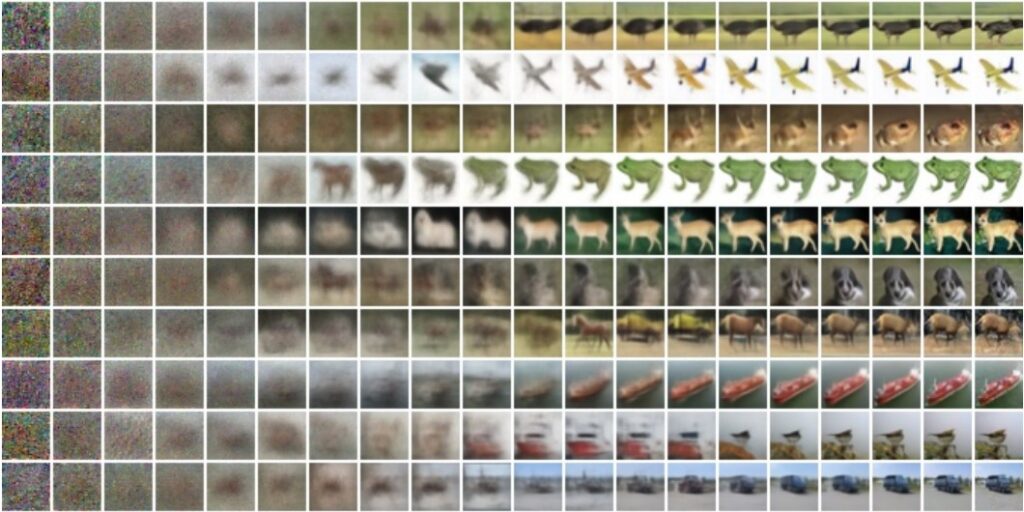
Repeatedly predict noise and take small denoising steps back toward data space.

Running this loop feels like watching static slowly coalesce into structure: blobs turn into silhouettes, silhouettes sharpen into objects, and textures and small details appear as $t$ approaches zero.

5. Practical Tips, Extensions, and Limitations

Implementing diffusion models from scratch is educational, but deploying them effectively requires attention to detail.

Conditioning is Key

A standard diffusion model without conditioning generates images that match the overall data distribution, but it cannot follow user instructions such as “generate a cat eating pizza.” To make the model controllable, you need conditioning.

You inject extra information (for example, text embeddings from a model such as CLIP) into the U-Net, usually via cross-attention layers or by concatenating features.
This guides the denoising process: “Remove the noise, but make sure the result looks like a cat eating pizza in the style of a watercolor painting.”

In practice, you can think of conditioning as an additional input channel of information that gently nudges each denoising step toward images that satisfy the prompt.

A widely used trick is classifier-free guidance: train the model sometimes with the condition (prompt) and sometimes with a “null” condition. At sampling time, combine the two predictions to trade off diversity versus prompt faithfulness. Another way to view this is that one model learns two behaviors, “denoise with condition” and “denoise unconditionally,” and sampling interpolates between them. At sampling time, you blend these two behaviors to trade off between faithfulness to the prompt (strong guidance) and sample diversity (weak guidance).

Schedulers Matter

The original DDPM process may require around $T = 1000$ reverse steps to generate an image, which is relatively slow.

DDIM (Denoising Diffusion Implicit Models): A faster sampling method that can generate high-quality images in as few as tens of steps by skipping parts of the reverse chain deterministically.
Euler Discrete / DPM-Solver: Modern solvers that treat the reverse process as solving a differential equation, often producing sharp images in 20–30 steps.

All of these schedulers reinterpret the reverse diffusion process as integrating a differential equation over time. Different solvers correspond to different integration schemes, exposing a speed-versus-quality trade-off without changing the underlying model. Libraries such as Hugging Face Diffusers expose these schedulers as interchangeable components, so you can trade off speed and sample quality without changing your core model.

Resolution and Latent Space

Generating high-resolution pixels (for example, $1024 \times 1024$) directly is computationally expensive and memory intensive.

Latent Diffusion (Stable Diffusion): Instead of running diffusion on pixel space, you use a Variational Autoencoder (VAE) to compress the image into a smaller latent space (for example, $64 \times 64$ feature maps). You then perform the diffusion process in this compressed space and use the VAE decoder to map the final latent back to an image.

Visually, you can imagine replacing a $512 \times 512$ RGB image with a much smaller grid of feature vectors, for example, $64 \times 64$ with 4 channels. Diffusion operates on this compact representation, which behaves like a semantic sketch of the image rather than raw pixels. This design dramatically reduces compute requirements while preserving perceptual quality, which is why it underpins many modern text-to-image systems.

Limitations and Considerations

Despite their strengths, diffusion models have practical downsides:

Sampling speed: Even with modern schedulers, you still need dozens of denoising steps, which can be slow compared with a single forward pass in a GAN.
Compute cost: Training high-resolution models from scratch is expensive (often many GPUs for days or weeks).
Data and biases: As with other generative models, outputs inherit biases from training data and can amplify them.
Control vs. diversity: Strong conditioning and guidance improve prompt adherence but can reduce diversity and sometimes introduce artifacts.
Reproducibility: Because sampling involves multiple stochastic steps, small changes in random seeds, schedulers, or guidance scales can lead to noticeably different outputs, which can complicate strict reproducibility.

How to Evaluate “Good” Samples

Diffusion models are often judged by images, but a technical viewpoint benefits from explicit metrics:

Fidelity: Are samples realistic (for example, measured by FID on a benchmark)?
Diversity: Do samples cover many modes (for example, precision/recall for generative models)?
Prompt adherence (conditional models): Does the output match the condition (human evaluation and task-specific metrics are common)?

Evaluation matters because improvements in sampling speed, guidance, or schedulers can change these trade-offs.

Conclusion

Diffusion models represent a paradigm shift in generative modeling. By learning the task of predicting and removing noise over many timesteps, they acquire a hierarchical notion of structure: coarse layout emerges early in the reverse process, while fine texture appears late.

In this article, we have explored three layers of the idea:

Intuition: a forward “fogging” process that gradually turns images into noise, and a learned reverse process that walks back toward clarity.
Mathematics: a Markov chain with Gaussian transitions, a tractable forward process $q(x_t | x_0)$, and a reverse process $p_\theta(x_{t-1} | x_t)$ trained via a simple noise-prediction objective.
Implementation: a concrete PyTorch setup with a noise schedule, a U-Net-style noise predictor, and a training loop that teaches the model to denoise across many noise levels.