Think of BERT as a strong, general-purpose “reader” that turns text into contextual vectors. The moment you move from a research notebook to the real world, you feel pressure from one of four directions:
- You want higher accuracy at the same input length.
- You need lower latency / smaller models for production.
- Your documents are long and $n^2$ attention becomes painful.
- Your text is specialized (biomedical, legal, finance), and generic pretraining becomes a liability.
Almost every BERT variant is a targeted response to one of these pressures. This note maps the landscape with a simple selection mindset: what changed, why it changed, and what you pay for it.
The Evolutionary Tree of Transformers
Think of BERT as a common ancestor. It uses an Encoder-only architecture, relies on Masked Language Modeling (MLM) and Next Sentence Prediction (NSP), and has an absolute limit of 512 tokens. It is accurate, but it is compute-heavy, memory-hungry, and strictly capped at 512 tokens. As this ancestor migrated into different environments—mobile phones, legal archives, hospital servers—it adapted.
We can organize these adaptations into a taxonomy based on what problem they solve.
A Taxonomy of BERT Variants
Instead of a random list of names, visualize these variants based on your primary bottleneck:
- Objective & Recipe (“Smarter” models): Models like RoBERTa and DeBERTa keep the size roughly the same but learn better by changing the pretraining rules.
- Distillation & Compression (“Faster” models): Models like DistilBERT, TinyBERT, and MobileBERT physically shrink the architecture to run faster on standard hardware or phones.
- Long-Context (“Wide-Angle” models): Models like Longformer and BigBird break the 512-token limit to read entire documents at once.
- Domain Specialists (“Experts” models): Models like BioBERT and LegalBERT are pretrained on specialized text to understand jargon that confuses the standard model.

Note: Longformer and BigBird are often described as Transformer encoder variants rather than strict “BERT variants”. Practically, they sit in the same workflow (tokenize → encoder → task head) and solve the same bottleneck (long documents).
Quick decision guide
- Best general accuracy (standard lengths): start with
roberta-baseor a DeBERTa checkpoint. - Strong quality per pretraining compute: consider
google/electra-base-discriminator. - Fast and small for serving: start with
distilbert-base-uncased; consider TinyBERT for more aggressive distillation. - Long documents ($>512$ tokens): use a long-context encoder such as Longformer or BigBird.
- Jargon-heavy domains: use a domain model (BioBERT, SciBERT, ClinicalBERT, LegalBERT, FinBERT, etc.).
- Many languages / cross-lingual: use XLM-R; consider distilled multilingual checkpoints for serving.
The “first question” checklist
Before comparing variants, answer these questions explicitly:
- Sequence length: do I live under 512 tokens, or not?
- Latency budget: do I need sub-50ms inference, or can I pay for a larger encoder?
- Domain shift: does my text contain heavy jargon or non-standard tokenization?
- Resources: do I have GPUs for fine-tuning and a rigorous evaluation loop?
1) Objective and Pretraining Recipe Variants (Better Learning Signal)
These variants mostly keep the Transformer encoder “shape” the same (12 layers, 768 hidden size), but they change how the model is exercised during training. It turns out that the exercises BERT did (Static Masking, Next Sentence Prediction) weren’t the most effective workout.
RoBERTa (Robustly Optimized BERT approach) [paper]
Core idea: keep the BERT architecture, change the training recipe.
- What changed
- Removes Next Sentence Prediction (NSP): It turned out that NSP was too easy. The model could often guess if sentence B followed sentence A just by checking if the topics matched (e.g., “clouds” and “weather”), without really understanding the grammar. Removing it forced the model to focus on the harder, “more nutritious” Masked Language Modeling task.
- Dynamic masking: BERT used static masks—the same sentence was always masked the same way. RoBERTa regenerates the mask every time it sees a sentence, preventing the model from just memorizing. For example, instead of using “The cat sat on the [MASK]” in all epochs, RoBERTa uses “The [MASK] sat on the mat” in epoch 1 and “The cat [MASK] on the mat” in epoch 11, and so on.
- Trains longer with bigger batches (batchsize increased from 256 to 8K) and more data.
- Uses a larger 50k BPE vocabulary containing subword units (byte-level BPE), which is cleaner than BERT’s character-level BPE (30k vocabulary).
- Notes
- The pretraining setup, not only the model, explains a large chunk of downstream performance.
- Similar inference cost to BERT (same Transformer encoder). Gains are mainly from better pretraining.
ALBERT (A Lite BERT) [paper]
Core idea: reduce parameters without (too much) accuracy loss.
- What changed
- Factorized embeddings: In standard BERT, the embedding layer is huge (vocab_size x hidden_size = $V \times H$). ALBERT splits this into two smaller matrices ($V \times E$ and $E \times H$).
- Instead of learning a massive, high-definition vector for every rare word, we learn a small “summary” vector, and then use a shared “projection” matrix to blow it up to the full hidden size. This helps the embedding layer to learn context-independent representations, whereas the projection layers learn context-dependent representations.
- Cross-layer parameter sharing: reuse the same Transformer layer (same attention and feed-forward weights) across all 12 layers.
- Standard BERT learns 12 specific steps. ALBERT learns one robust step and applies it 12 times recursively.
- Replaces NSP with Sentence Order Prediction (SOP). That is, given two consecutive segments A and B from the corpus, the model predicts whether B follows A or not. This focuses on inter-sentence coherence rather than mere relatedness.
- Factorized embeddings: In standard BERT, the embedding layer is huge (vocab_size x hidden_size = $V \times H$). ALBERT splits this into two smaller matrices ($V \times E$ and $E \times H$).
- Notes
- Much smaller parameter footprint, often comparable performance on many tasks.
- Better suited for memory-constrained scenarios.
- Parameter sharing can reduce representational diversity across layers.
- Speedups depend on implementation; fewer parameters does not always imply proportionally faster inference.
ELECTRA (Efficiently Learning an Encoder that Classifies Token Replacements Accurately) [paper]
Core idea: make pretraining more sample-efficient than masked language modeling.
- What changed
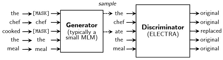
- Replaced Token Detection (RTD): Instead of
[MASK], tokens are replaced by plausible alternatives sampled from a small generator network. - Discriminator Loss: The model predicts a binary label (Original vs. Replaced) for every token. Thus, instead of predicting masked tokens, ELECTRA trains a discriminator that predicts whether each token is original or replaced.
- A small generator (a small criminal model) proposes replacements; the discriminator (our main model) learns from all token positions.
- Replaced Token Detection (RTD): Instead of
- Notes
- BERT learns from MLM, which provides learning signal only on masked positions (often 15%). ELECTRA provides signal on (almost) every token.
- For a fixed compute budget, ELECTRA often yields stronger downstream results.
- Pretraining is more complex (two networks, careful balancing).
- The discriminator objective is different from generation; it is primarily for representation learning.
DeBERTa (Decoding-Enhanced BERT with disentangled Attention) [paper]
Core idea: represent content and position separately.
- What changed
- Disentangled Attention: Standard BERT adds the content embedding and position embedding into a single vector (like mixing red and blue paint to make purple). You can’t un-mix them. DeBERTa keeps them separate. It calculates attention scores using separate matrices for “content-to-content” and “content-to-position”. This allows the model to distinguish “how related are these two words?” from “how far apart are they?” much more clearly.
- Introduces relative position handling that can improve generalization.
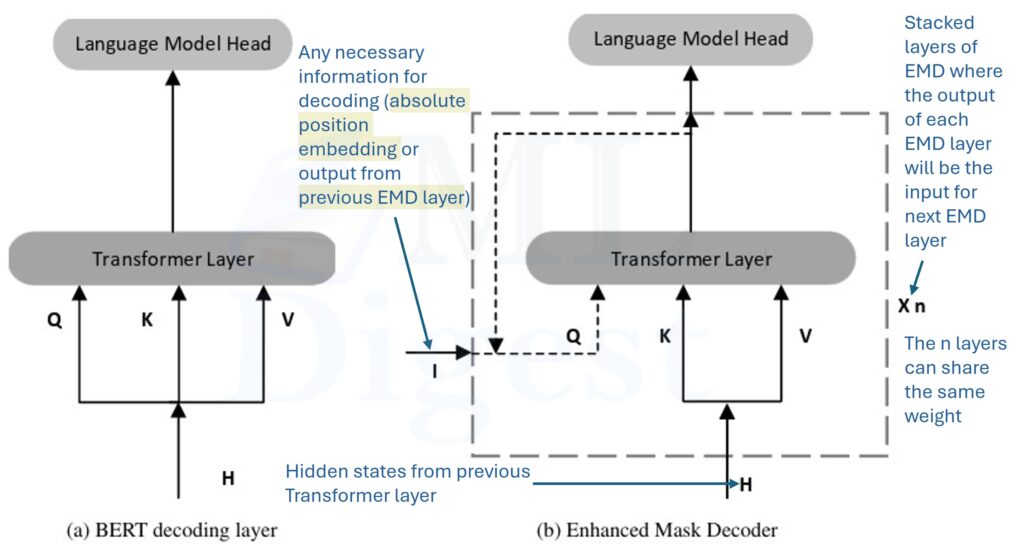
- Enhanced Mask Decoder (EMD): adds an auxiliary decoding task during pretraining to better reconstruct masked tokens.
- Notes
- Better modeling of word order and relative structure without forcing position and content into a single embedding.
- More complex attention computation.
SpanBERT (Span-Level Masking) [paper]
Core idea: Instead of masking random individual words ([MASK]), mask contiguous spans ([MASK] [MASK] [MASK]). This forces the model to use context from the edges to predict the middle.
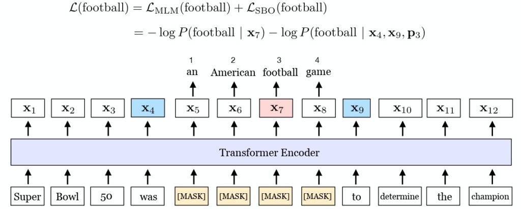

(This figure depicts the training process of SpanBERT. The phrase “an American football game” is masked out. To recover the masked content, the span boundary objective (SBO) relies on the output representations of the boundary tokens $x_4$ and $x_9$ (highlighted in blue) to predict the tokens inside the span. The equation illustrates the MLM and SBO loss components for predicting the word “football”, which is indicated by the position embedding $p_3$ as the third token following $x_4$. Source: SpanBERT paper)
- What changed
- Replaces token-level random masks with contiguous span masks.
- Adds objectives that better support span-based tasks.
- Notes
- Improves performance on tasks where spans matter: question answering, coreference, information extraction.
- Mainly a pretraining difference; inference cost remains BERT-like.
2) Distillation and Compression Variants (Better Serving)
When deploying models to production, size and speed matter. You often cannot afford the latency of a full 12-layer BERT. This is where Knowledge Distillation comes in.
DistilBERT [paper]
Core idea: train a smaller student model to mimic a larger teacher (BERT).
- What changed
- Layer Pruning: DistilBERT takes a 12-layer BERT, removes every other layer, and initializes the remaining 6 layers from the teacher.
- Distillation Loss: It optimizes a triple loss: (1) Soft target loss (mimicking the teacher), (2) Masked Language Modeling loss (mimicking the data), and (3) Cosine embedding loss (aligning vector directions).
- Notes
- Strong speed improvements (about 60% faster) and size reductions (about 40% smaller), with modest accuracy drop (97% of original).
- Popular default for production when full BERT is too heavy.
- Reduced capacity can hurt tasks needing deep reasoning or long context.
TinyBERT[paper]; MobileBERT [paper]
Core idea: distillation plus architecture choices aimed at mobile/edge.
- TinyBERT
- Emphasizes layer-wise distillation and intermediate representation matching.
- The training method introduces three categories of loss functions, each targeting a different level of representation within BERT: (1) the outputs of the embedding layer, (2) the hidden states and attention matrices produced by the Transformer layers, and (3) the logits generated by the prediction layer.
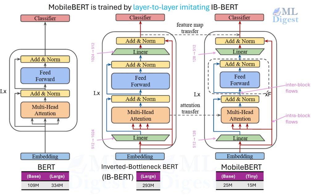
- MobileBERT
- Engineers a bottleneck structure and training recipe designed for mobile inference.
- As shown in below image, MobileBERT is distilled from a specially designed teacher model called Inverted Bottleneck BERT (IB-BERT). The IB-BERT architecture introduces bottleneck structures within the Transformer layers, which increases the dimensionality of the intermediate representations. This design choice improves efficiency and performance. The distillation process involves training MobileBERT to mimic the outputs and internal representations of the IB-BERT teacher model, ensuring that despite its compact size, MobileBERT retains high performance on downstream tasks.
- Notes
- MobileBERT achieves near-BERT accuracy while being 4.3x smaller and 5.5x faster than BERT.
- May require careful choice of pretraining and fine-tuning to preserve accuracy.
3) Long-Context Encoder Variants (Long Documents)
Vanilla self-attention is $O(n^2)$ complexity. If you double the text length, the memory usage quadruples. At 512 tokens, it’s fine. At 4,000 tokens, your GPU runs out of memory (OOM). Long-context encoders typically reduce this cost via sparsity (limit which tokens can attend to which), and some related models extend context via recurrence/caching.
The Intuition (Sparse Attention):
Imagine a cocktail party.
- Dense Attention (BERT): Everyone talks to everyone else simultaneously. It is loud and chaotic. (Cost grows nicely with 10 people, explodes with 1,000).
- Sliding Window (Longformer): You only talk to the 5 people to your left and right.
- Global Tokens (Longformer/BigBird): A few “moderators” (the
[CLS]token) stand on a stage. Everyone can hear the moderator, and the moderator can hear everyone. To send a message to the other side of the room, you pass it to the moderator.
Longformer [paper]
Core idea: use a combination of local (sliding-window) attention and a small set of global attention patterns to scale self-attention to long sequences while preserving important cross-sequence interactions.
- What changed
- Replaces the dense $O(n^2)$ attention with a sliding-window (local) attention: each token attends to a fixed-size window of neighbors (size w). This reduces complexity to $O(nw)$.
- To increase the receptive field without increasing computational overhead, the authors introduce a dilated sliding window.
- Introduces global attention for a small number of tokens (for example special classification tokens like
[CLS]or document-level markers). Global tokens can attend to all tokens and all tokens can attend to them. - Implements the local window efficiently using masked attention and attention pattern sparsity so that existing Transformer implementations can be adapted with modest engineering effort.
- LED (Longformer-Encoder-Decoder) is a variant of the Longformer model specifically designed to support generative sequence-to-sequence (seq2seq) learning for long documents.

- Notes
- Enables processing of much longer inputs (thousands of tokens) with linear-ish cost in practice.
- Preserves local contextual modeling via the window and global information flow via global tokens, which is crucial for tasks like long-document classification, QA over long contexts, and summarization.
- Time and memory complexity become $O(nw + ng)$ where $w$ is the window size and $g$ is the number of global tokens (usually small), instead of $O(n^2)$.
- Empirically, Longformer matches or exceeds baseline models on long-document tasks while remaining efficient.
- The paper shows how to compose windowed attention with global attention and describes a flexible API for combining patterns (local + global + dilated variants).
flowchart TB
    subgraph Dense[Dense attention]
        A1[Token i] --> A2[All tokens]
    end
    subgraph Sparse["Longformer"]
        B1[Token i] --> B2["Window neighbors (w)"]
        B1 --> B3["Global tokens (g)"]
        B3 --> B4[All tokens]
    end
BigBird [paper]
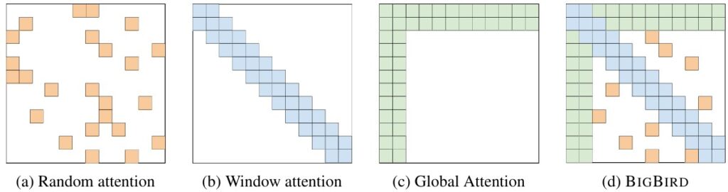
Core idea: sparse attention with a combination of random, local, and global patterns.
- What changed
- Attention edges = local window + random connections + global tokens.

- Notes
- Better theoretical coverage and empirical performance on long documents.
- More complex attention pattern; tuning can matter.
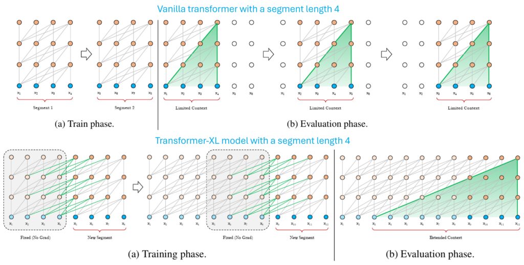
Transformer-XL (Related Family) [paper]
Transformer-XL is not strictly a “BERT variant”, but it influenced long-context strategies via recurrence and caching past states.
- Key idea
- Carry hidden states across segments to extend effective context. That is, when processing segment $t$, the model can attend to cached hidden states from segment $t-1$.
- Proposes a novel relative positional encoding scheme.
- Notes
- Enables learning longer-term dependencies beyond fixed-length segments.
- Different from sparse attention; more about reusing past computations.
4) Domain-Specific BERTs (Better Match)
Core idea: keep the architecture, change the pretraining corpus (and sometimes vocabulary).
- BioBERT: biomedical papers (PubMed, PMC). [paper]
- ClinicalBERT: clinical notes (often derived from MIMIC-style text). [paper]
- SciBERT: scientific papers across domains; often comes with a science-specific vocabulary. [paper]
- The same pattern applies in legal, financial, patent, and other specialized domains (LegalBERT: [paper]; FinBERT: [paper]).
Notes
- If your text is jargon-heavy and labeled data is limited, a domain BERT usually helps.
- Domain terms (“IL-6”, “BRCA1”, “meta-analysis”, “p-value”, “HbA1c”) get better tokenization and embeddings.
- Improves named entity recognition, relation extraction, literature mining, and clinical coding tasks.
- Domain models can underperform on general text.
- Vocabulary changes can make cross-domain transfer more awkward.
5) Multilingual and Cross-Lingual Variants
mBERT (Multilingual BERT) [paper], code, model
Core idea: train one model on many languages with a shared subword vocabulary. Enables zero-shot or low-shot cross-lingual transfer: fine-tune on English, test on another language (sometimes surprisingly well).
XLM-R (Cross-lingual Language Model RoBERTa) [paper]
Core idea: RoBERTa-style training at multilingual scale. Often stronger than mBERT due to more data and tuned recipe.
6) “Whole-Word”, “Cased/Uncased”, and Tokenization Variants
These are not always separate papers, but they matter in practice.
Whole Word Masking (WWM)
- What changed
- If a word splits into subwords, mask all of its subwords together.
- Notes
- Encourages learning word-level semantics rather than only subword completion.
Cased vs Uncased
- Cased models preserve capitalization; often better for named entities.
- Uncased models can be more robust to messy text but may lose signals.
Vocabulary Differences
- Changing the tokenizer (WordPiece vs SentencePiece) can change out-of-vocabulary behavior and multilingual coverage.
In practice, tokenizer differences are one of the most common sources of “silent failure” when swapping checkpoints.
7) Comparison Table (What You Pay For What You Get)
This table is intentionally high-level. Confirm details against the exact checkpoint you use.
| Variant | Main change | Primary benefit | Common trade-off |
|---|---|---|---|
| RoBERTa | Better recipe, no NSP | Stronger accuracy | Same inference cost as BERT |
| ALBERT | Parameter sharing, factorized embeddings | Fewer parameters | May reduce layer diversity |
| ELECTRA | Replaced-token detection | More sample-efficient pretraining | More complex pretraining setup |
| DeBERTa | Disentangled attention | Strong accuracy, better positional modeling | More complex attention |
| SpanBERT | Span masking | Better span-centric tasks | Same inference cost |
| DistilBERT | Distillation | Faster, smaller | Some accuracy loss |
| MobileBERT | Mobile-friendly architecture + distillation | Edge deployment | Recipe complexity |
| Longformer | Sparse attention | Longer context | Task-dependent global token design |
| BigBird | Sparse attention pattern mix | Long documents | More tuning complexity |
| BioBERT/SciBERT/etc. | Domain corpus | Better in-domain NLP | Can degrade on general text |
| mBERT/XLM-R | Multilingual corpus | Cross-lingual transfer | Capacity diluted across languages |
If you are undecided, a strong default pairing is: distilbert-base-uncased for constrained serving, and roberta-base for higher accuracy at standard lengths.
8) Practical Workflow: How to Compare Variants Fairly
Most “model comparisons” become unfair because multiple variables change at once. A simple workflow that usually produces reliable conclusions is:
- Fix the task and data split (exact same train/validation/test).
- Fix the training budget first (same epochs, same max steps, same batch size).
- Keep the tokenizer paired with the checkpoint (never mix weights and tokenizer).
- Measure accuracy and cost (latency, memory, throughput), not only accuracy.
- Only then do model-specific tuning (learning rate, warmup, max length).
By following this procedure, you can isolate the effect of the model variant itself rather than confounding factors when building your own custom model.
9) What Changed Mathematically
Most BERT-like encoders compute self-attention as:
$$
\mathrm{Attention}(Q, K, V) = \mathrm{softmax}\left(\frac{QK^T}{\sqrt{d}}\right)V
$$
Variants often modify either:
- How $Q, K, V$ are produced (parameter sharing in ALBERT, bottlenecks in MobileBERT)
- How position information is injected (relative positions, disentangled attention in DeBERTa)
- Which tokens attend to which (sparse patterns in Longformer/BigBird)
- What loss is used in pretraining (ELECTRA discriminator vs MLM)
Common Pitfalls
- Mask token mismatch: BERT uses
[MASK], RoBERTa uses<mask>. - Tokenizer mismatch across checkpoints: do not mix and match tokenizers and weights.
- Sequence length assumptions: many checkpoints were pretrained with a certain max length; extending length is not just a config change.
- Domain shift: a domain BERT can outperform general BERT dramatically in-domain, but degrade out-of-domain.
Conclusion
The BERT ecosystem looks crowded until you classify models by the pressure they are responding to: accuracy, efficiency, length, or domain mismatch. Once you frame your constraints (sequence length, latency budget, and domain shift), the variant choice becomes a constrained engineering decision rather than a naming contest.
If you want a robust default workflow: pick one strong baseline (RoBERTa or DeBERTa at standard length; Longformer or BigBird for long documents; DistilBERT for strict latency), then evaluate fairly with fixed data splits and budgets.

Happy is a seasoned ML professional with over 15 years of experience. His expertise spans various domains, including Computer Vision, Natural Language Processing (NLP), and Time Series analysis. He holds a PhD in Machine Learning from IIT Kharagpur and has furthered his research with postdoctoral experience at INRIA-Sophia Antipolis, France. Happy has a proven track record of delivering impactful ML solutions to clients.
Subscribe to our newsletter!