What is Batch Normalization and Why is it Important?

Batch normalization was introduced in 2015. By normalizing layer inputs, batch normalization helps to stabilize and accelerate the training process, leading to faster convergence and improved performance.

Normalization in Neural Networks

Normalization refers to techniques that adjust and scale the input data to ensure that it fits within a specific range or distribution. In the context of neural networks, normalization is typically applied to the activations of layers or to the inputs. Proper normalization can stabilize and accelerate training, leading to better performance.

Before batch normalization, techniques like input normalization (e.g., scaling pixel values between 0 and 1) and weight initialization strategies were commonly used to facilitate training. Batch normalization extends the concept of normalization to the activations within the network layers, addressing additional challenges related to internal covariate shift.

Motivations Behind Batch Normalization

Training deep neural networks involves optimizing a highly non-convex loss function. Several factors can hinder effective optimization:

1. Internal Covariate Shift: As training progresses, the distribution of activations in each layer changes due to updates in previous layers. This shift forces layers to continuously adapt to new distributions, slowing down training.
2. Vanishing/Exploding Gradients: Poorly scaled activations can result in gradients that either diminish to near zero or explode to large values, making optimization difficult.
3. Sensitivity to Initialization: Networks without proper normalization are highly sensitive to weight initialization schemes.

Batch normalization addresses these issues by stabilizing the distribution of activations, allowing for more effective and faster training.

What is Batch Normalization?

Batch normalization is a technique to normalize the inputs of each layer within a neural network. Specifically, it normalizes the activations of the previous layer for each mini-batch, ensuring that they have a mean of zero and a variance of one. This normalization is performed separately for each feature dimension.

How Batch Normalization Works

(Image credit: Medium post)

Batch normalization can be applied to various types of layers, including fully connected and convolutional layers.

1. Mini-Batch Collection: During training, data is processed in mini-batches. Batch normalization computes statistics (mean and variance) over each mini-batch.
2. Normalization: For each feature in the mini-batch, compute the mean and variance, and normalize the activations accordingly.
3. Scaling and Shifting: Apply the learned parameters \( \gamma \) and \( \beta \) to allow the network to recover the representation it would have learned without normalization.
4. Propagation: The normalized and scaled activations are then passed to the next layer.
5. Parameter Updates: Both the network weights and the batch normalization parameters \(( \gamma \) and \( \beta \)) are updated during backpropagation.

During training, batch normalization uses the statistics of the current mini-batch. However, during inference (testing or deployment), it uses running averages of the statistics collected during training to ensure consistent behavior.

During Training

Batch normalization introduces two trainable parameters for each feature: a scaling factor \(\gamma\) and a shift factor \(\beta\). These parameters allow the network to maintain the representational power it had without normalization.

Given a mini-batch (with mini batch-size \(m\) ) of activations \( {x^{(1)}, x^{(2)}, \dots, x^{(m)}} \) for a particular neuron in a layer:

1. Compute the Mini-Batch Mean:
   \[
   \mu_{\text{batch}} = \frac{1}{m} \sum_{i=1}^{m} x^{(i)}
   \]
2. Compute the Mini-Batch Variance:
   \[
   \sigma^2_{\text{batch}} = \frac{1}{m} \sum_{i=1}^{m} (x^{(i)} – \mu_{\text{batch}})^2
   \]
3. Normalize:
   \[
   \hat{x}^{(i)} = \frac{x^{(i)} – \mu_{\text{batch}}}{\sqrt{\sigma^2_{\text{batch}} + \epsilon}}
   \]
   Here, \( \epsilon \) is a small constant added for numerical stability.
4. Scale and Shift:
   \[
   y^{(i)} = \gamma \hat{x}^{(i)} + \beta
   \]
   \( \gamma \) and \( \beta \) are learnable parameters.

During Inference

During inference, batch normalization must use consistent statistics since there may be only one sample or varying batch sizes:

1. Use Running Statistics: Instead of batch statistics, use the running mean and variance accumulated during training.
2. Normalization and Scaling: Normalize using the running mean and variance, then apply \( \gamma \) and \( \beta \).

This distinction ensures that the model’s behavior is deterministic during inference, regardless of batch size. Most deep learning frameworks handle this automatically, but it is important to be aware of the distinction.

Benefits of Batch Normalization

Batch normalization offers several advantages that contribute to more efficient and effective neural network training:

1. Stabilizes Learning Process: By maintaining consistent activation distributions, batch normalization reduces the fluctuations in the network’s internal representations.
2. Accelerates Training: Networks with batch normalization can often be trained with higher learning rates, leading to faster convergence.
3. Reduces Sensitivity to Initialization: The normalization makes the network’s performance less dependent on the initial weight distribution, allowing for more straightforward initialization strategies.
4. Acts as a Regularizer: The noise introduced by mini-batch statistics can have a regularizing effect, potentially reducing the need for other forms of regularization like dropout.
5. Mitigates Vanishing/Exploding Gradients: By controlling the scale of activations, batch normalization helps in maintaining healthy gradient flow during backpropagation.
6. Enables Deeper Networks: With more stable gradients and activations, it becomes feasible to train deeper architectures without degradation in performance.

Practical Tips

To effectively leverage batch normalization in neural network training, consider the following best practices:

1. Placement: Insert batch normalization layers after the linear transformations (e.g., fully connected or convolutional layers) and before the activation functions. For example:

   [Linear Layer] -> [Batch Norm] -> [Activation Function]  

2. Initialization of \( \gamma \) and \( \beta \): Initialize \( \gamma \) to 1 and \( \beta \) to 0. This setup ensures that the network initially passes through the normalized activations unaltered.
3. Use of Higher Learning Rates: With batch normalization stabilizing the training process, it’s often beneficial to use higher learning rates, potentially reducing training time.
4. Mini-Batch Size Considerations: Batch normalization relies on mini-batch statistics. Extremely small batch sizes can lead to poor estimates of mean and variance. In such cases, consider alternatives like layer normalization or group normalization.
5. Handling Dropout: If using dropout as a regularization technique, place batch normalization before dropout layers. This sequencing ensures that the activations are normalized before being randomly dropped.
6. Inference Mode: Ensure that during inference, the normalization layer switches to using the running averages instead of batch statistics.

Example in TensorFlow

import tensorflow as tf  
   
model = tf.keras.models.Sequential([  
    tf.keras.layers.Dense(128, input_shape=(784,)),  
    tf.keras.layers.BatchNormalization(),  
    tf.keras.layers.Activation('relu'),  
    tf.keras.layers.Dense(64),  
    tf.keras.layers.BatchNormalization(),  
    tf.keras.layers.Activation('relu'),  
    tf.keras.layers.Dense(10, activation='softmax')  
])  
   
model.compile(optimizer='adam',  
              loss='sparse_categorical_crossentropy',  
              metrics=['accuracy'])  
              

Example in PyTorch

import torch  
import torch.nn as nn  
   
class SimpleNN(nn.Module):  
    def __init__(self):  
        super(SimpleNN, self).__init__()  
        self.fc1 = nn.Linear(784, 128)  
        self.bn1 = nn.BatchNorm1d(128)  
        self.fc2 = nn.Linear(128, 64)  
        self.bn2 = nn.BatchNorm1d(64)  
        self.fc3 = nn.Linear(64, 10)  
  
    def forward(self, x):  
        x = torch.relu(self.bn1(self.fc1(x)))  
        x = torch.relu(self.bn2(self.fc2(x)))  
        x = self.fc3(x)  
        return x  
   
model = SimpleNN()  
   
criterion = nn.CrossEntropyLoss()  
optimizer = torch.optim.Adam(model.parameters(), lr=0.001)  

Limitations and Considerations

While batch normalization offers substantial benefits, it’s essential to be aware of its limitations:

1. Dependency on Mini-Batch Statistics: The effectiveness of batch normalization diminishes with very small batch sizes, as the estimated statistics become unreliable.
2. Incompatibility with Certain Architectures: Some architectures, like generative adversarial networks (GANs), where batch statistics can leak information between the generator and discriminator, may require careful handling or alternative normalization strategies.
3. Additional Computational Overhead: Batch normalization introduces extra computations and parameters, which can marginally increase training time and memory usage.
4. Non-Applicability to Certain Tasks: Tasks that require instance-specific outputs, such as certain types of reinforcement learning, may not benefit from batch normalization.
5. Increased Complexity During Deployment: Proper handling of mode switching between training and inference is crucial. Mistakes here can lead to degraded performance.

Variations and Extensions

(Image credit: AI Summer blog)

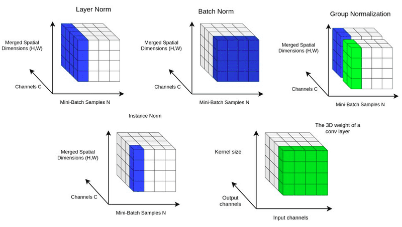
1. Layer Normalization: Normalizes across features for each data sample, independent of the batch size.
2. Instance Normalization: Normalizes each feature map individually, commonly used in style transfer.
3. Group Normalization: Divides channels into groups and normalizes within each group, offering flexibility across varying batch sizes.
4. Batch Renormalization: Enhances batch normalization by better approximating population statistics during training.
5. Switchable Normalization: Allows the network to learn the optimal combination of different normalization methods dynamically.
6. Weight Normalization: Normalizes the weights of layers instead of activations, decoupling the direction and magnitude of weight vectors.

Each alternative has its use cases and advantages, and the choice often depends on the specific requirements of the task and the architecture.

Concluding Remarks

By stabilizing the distribution of activations, Batch normalization enables faster convergence, mitigates issues like internal covariate shift, and often enhances generalization performance. Its integration into various architectures underscores its versatility and effectiveness.

Refesources

• Ioffe, S., & Szegedy, C. (2015). Batch Normalization: Accelerating Deep Network Training by Reducing Internal Covariate Shift. arXiv:1502.03167.
• AI Summer blog
• Medium post