Adjusted R-Squared: Why, When, and How to Use It

Adjusted R-squared is one of those metrics that shows up early in regression, but it often feels like a small correction to regular R-squared. In practice, it encodes an important idea:

Do not reward a model just because it has more features.

This note walks through the intuition, the math, and how adjusted R-squared behaves in realistic machine learning workflows.

Quick Intuition

Imagine you are building a linear regression model to predict house prices:

You start with 2 features: living area and number of bedrooms.
You then keep adding more features: zip-codes, interaction terms, polynomial terms, and even random noise.

Regular R-squared almost always goes up (or stays the same) when you add more features, even if these features are useless. It answers:

“How much of the variance in the target can my model explain, given all the features it already has?”

It does not ask whether those features were necessary or actually helpful.

Adjusted R-squared adds this missing question:

“Is this improvement in fit large enough to justify the extra complexity?”

You can think of adjusted R-squared as a penalized version of R-squared:

If a new feature genuinely helps, adjusted R-squared will increase.
If a new feature is just noise or redundant, adjusted R-squared will decrease.

So adjusted R-squared behaves like a cautious teammate who keeps asking: “Are these extra features really paying rent?”

Recap: Ordinary R-Squared

Before defining adjusted R-squared, let us recall ordinary R-squared.

Consider a regression problem with:

$n$ observations,
a continuous target $y$, and
predictions $\hat{y}$ from a regression model.

Define:

Total Sum of Squares ($SS_{tot}$): overall variation in $y$ $$
SS_{tot} = \sum_{i=1}^n (y_i – \bar{y})^2
$$ where $\bar{y}$$ is the mean of $y$.
Residual Sum of Squares ($SS_{res}$): unexplained variation left after fitting the model
$$ {SS}_{res} = \sum_{i=1}^n (y_i – \hat{y}_i)^2 $$

Then R-squared is

$$ R^2 = 1 – \frac{{SS}_{res}}{{SS}_{tot}} $$

Interpretation:

$R^2$ is the fraction of variance explained by the model.
$R^2 = 0$: the model is no better than predicting the mean $\bar{y}$.
$R^2 = 1$: the model fits the data perfectly ($SS_{res} = 0$).

The Key Limitation

If you keep adding features, ${SS}_{res}$ never increases. At worst, the model can ignore a feature. As a result:

$R^2$ never decreases when you add predictors.
A huge model with many useless features can have a high $R^2$ simply by overfitting the training data.

Relying on $R^2$ alone can mislead you into preferring unnecessarily complex models.

Definition of Adjusted R-Squared

Adjusted R-squared modifies $R^2$ with a penalty term that depends on:

the number of observations $n$, and
the number of predictors (features) $p$ in the model.

Formally, for a linear regression with intercept:

$$
R^2_{\text{adj}} = 1 – \biggl(1 – R^2\biggr) \cdot \frac{n – 1}{n – p – 1}.
$$

Equivalently, using $SS_{res}$ and $SS_{tot}$ directly:

$$
R^2_{\text{adj}} = 1 – \frac{SS_{res} / (n – p – 1)}{SS_{tot} / (n – 1)}.
$$

Here:

$n$ = number of samples,
$p$ = number of predictors (excluding the intercept),
$n – p – 1$ = residual degrees of freedom.

The fraction $\frac{{SS}{res}}{n – p – 1}$ is the unbiased estimate of the residual variance, while $\frac{{SS}{tot}}{n – 1}$ is the sample variance of $y$.

So adjusted R-squared can be seen as

1 minus the ratio of estimated residual variance to target variance.

This connects directly to the intuition: you wish to compare how much variance is left after fitting the model, while accounting for how many parameters were used to get that fit.

How the Penalty Works

Let us unpack the penalty term

$$
\frac{n – 1}{n – p – 1}.
$$

Behavior as Features Increase

When you add more predictors (increase $p$), the denominator $n – p – 1$ shrinks.
The ratio $\frac{n – 1}{n – p – 1}$ therefore grows.
This amplifies the term $(1 – R^2)$, which reduces $R^2_{\text{adj}}$.

For adjusted R-squared to increase after adding a predictor, the new feature must reduce ${SS}_{res}$ enough so that the decrease in $(1 – R^2)$ outweighs the growth in the penalty.

This effect is especially strong when:

$n$ is small, and
$p$ is large compared to $n$.

In that setting, models are prone to overfitting, and adjusted R-squared becomes more conservative.

Can Adjusted R-Squared Be Negative?

Yes. adjusted $R^2$ can be negative.

If your model performs worse than predicting the mean, then ${SS}_{res} > {SS}_{tot}$,
and the penalty factor can push $R^2_{\text{adj}}$ below 0.

A negative adjusted R-squared says: “Given your number of features, you are doing worse than a trivial baseline.”

Worked Example (Conceptual)

Assume you have $n = 100$ observations.

Model A: 2 Features

$p = 2$
$R^2 = 0.80$

Then

$$
R^2_{\text{adj}} = 1 – (1 – 0.80) \cdot \frac{100 – 1}{100 – 2 – 1}
\approx 1 – 0.2041
\approx 0.796.
$$

So adjusted $R^2$ is slightly lower than $R^2$.

Model B: 50 Features

Now suppose you add many features and get:

$p = 50$
$R^2 = 0.90$ (seems much better at first glance)

Then

$$
R^2_{\text{adj}} = 1 – (1 – 0.90) \cdot \frac{100 – 1}{100 – 50 – 1}
\approx 1 – 0.2020
\approx 0.798.
$$

Despite a large jump in $R^2$ (from 0.80 to 0.90), adjusted $R^2$ improves only slightly (from about 0.796 to about 0.798).

Interpretation:

The huge increase in complexity (from 2 to 50 features) bought you very little “explained variance per parameter.”
Adjusted R-squared reflects this trade-off and refuses to reward this model aggressively.

In practice, you might prefer Model A (simpler, more interpretable) unless there is a strong domain reason to keep the additional features.

Adjusted R-Squared vs R-Squared

You can summarize the differences as follows:

R-squared
- Measures goodness of fit on the training data.
- Never decreases when new predictors are added.
- Can be overly optimistic for models with many features.
Adjusted R-squared
- Measures goodness of fit per degree of freedom.
- Can decrease when new predictors do not improve the model enough.
- Encourages parsimonious models with fewer, more informative features.

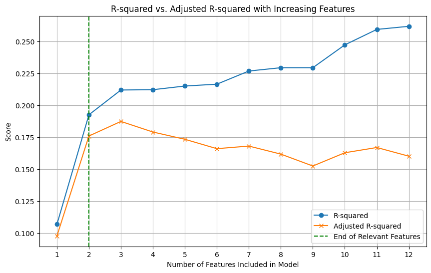
Plotting both curves against the number of features makes the trade-off transparent: $R^2$ starts low and monotonically increases as features are added — it may flatten but never turns down — whereas adjusted $R^2$ typically rises only while truly informative predictors are added, reaches a peak at an optimal feature count, and then declines as extra predictors contribute more noise than signal; that peak therefore provides a simple, practical heuristic for choosing a parsimonious model in classical regression, to be used alongside residual diagnostics and domain knowledge.

In regression modeling, it is common to report both:

$R^2$ to show raw explained variance,
$R^2_{\text{adj}}$ to show variance explained after accounting for complexity.

When to Use Adjusted R-Squared

Adjusted R-squared is particularly useful when:

You are working with linear or generalized linear models.
You are comparing nested models (one model is a special case of another with fewer predictors).
You want a single-number summary that balances fit and complexity.

Typical use cases:

Feature selection in linear regression
- Compare models with different subsets of features.
- Prefer the model with the highest adjusted $R^2$, provided assumptions are reasonable.
Model reporting
- In econometrics or classical statistics papers, adjusted $R^2$ is commonly reported as a quality-of-fit indicator.

When Not to Rely on It

Avoid over-relying on adjusted R-squared when:

The model is non-linear or highly flexible (e.g., random forests, gradient boosting, deep networks).
The regression assumptions are strongly violated.
You care primarily about out-of-sample performance, in which case:
- Use a held-out validation set.
- Or use cross-validation and metrics like RMSE, MAE, or predictive $R^2$ on validation folds.

Adjusted R-squared is best viewed as a classical linear-model diagnostic, not a universal model selection metric.

Why Adjusted $R^2$ Does Not Apply to Random Forests

Adjusted $R^2$ was created for parametric linear models, where:

The model has a fixed, known number of parameters (e.g., number of predictors)
Adding predictors always increases $R^2$, even if they are useless
Adjusted $R^2$ penalizes model complexity.

Why this breaks for Random Forests?

Random Forests are non-parametric ensemble models:

No clear $p$: RFs do not have a well-defined number of parameters
Complexity ≠ #features: Complexity depends on trees, depth, splits, bootstrapping
Feature reuse: Same feature can be used many times across trees
Overfitting already handled: RFs reduce overfitting via bagging

So, plugging in $p =$ number of features is theoretically incorrect and plugging in number of nodes/trees is arbitrary, leading to misleading adjusted $R^2$ values with no clear statistical meaning.

Adjusted R-Squared in Practice (Python)

Let us now connect the theory to a small, runnable example in Python using scikit-learn. The goal is to show how ordinary and adjusted R-squared behave when you add irrelevant features.

Python

import numpy as np

# 2. Set a random seed for reproducibility
np.random.seed(12)

# 3. Define the number of samples
n_samples = 100

# 4. Define the number of relevant features
n_relevant = 2

# 5. Define the number of irrelevant features
n_irrelevant = 10

# 6. Generate n_relevant features for X_relevant
X_relevant = np.random.rand(n_samples, n_relevant)

# 7. Generate n_irrelevant features for X_irrelevant
X_irrelevant = np.random.rand(n_samples, n_irrelevant)

# 8. Define coefficients for the relevant features and an intercept
true_coefficients = np.array([2, -1.5]).reshape(-1, 1)
intercept = 5

# 9. Generate the target variable y
y = intercept + X_relevant @ true_coefficients + np.random.randn(n_samples, 1) * 2

# 10. Combine X_relevant and X_irrelevant horizontally to create the full feature matrix X
X = np.hstack((X_relevant, X_irrelevant))

# 11. Print the shapes of X and y to verify the generated data dimensions
print(f"Shape of X: {X.shape}")
print(f"Shape of y: {y.shape}")


from sklearn.linear_model import LinearRegression
from sklearn.metrics import r2_score
import numpy as np

# Initialize lists to store results
r2_values = []
adj_r2_values = []

n_samples = X.shape[0]

# Loop through features, first relevant, then irrelevant
for i in range(1, X.shape[1] + 1):
    # Select subset of features
    # The first n_relevant features are relevant, the rest are irrelevant
    X_subset = X[:, :i]

    # Fit a Linear Regression model
    model = LinearRegression()
    model.fit(X_subset, y)

    # Make predictions
    y_pred = model.predict(X_subset)

    # Calculate R-squared
    r2 = r2_score(y, y_pred)
    r2_values.append(r2)

    # Calculate Adjusted R-squared
    n_features = X_subset.shape[1]
    # Handle case where (n_samples - n_features - 1) might be 0 or negative
    if (n_samples - n_features - 1) <= 0:
        adj_r2 = np.nan # Or some other appropriate value for invalid calculation
    else:
        adj_r2 = 1 - ((1 - r2) * (n_samples - 1) / (n_samples - n_features - 1))
    adj_r2_values.append(adj_r2)

print("R-squared values for models with increasing features:", [f'{val:.4f}' for val in r2_values])
print("Adjusted R-squared values for models with increasing features:", [f'{val:.4f}' if not np.isnan(val) else 'NaN' for val in adj_r2_values])

import numpy as np

# 2. Set a random seed for reproducibility
np.random.seed(12)

# 3. Define the number of samples
n_samples = 100

# 4. Define the number of relevant features
n_relevant = 2

# 5. Define the number of irrelevant features
n_irrelevant = 10

# 6. Generate n_relevant features for X_relevant
X_relevant = np.random.rand(n_samples, n_relevant)

# 7. Generate n_irrelevant features for X_irrelevant
X_irrelevant = np.random.rand(n_samples, n_irrelevant)

# 8. Define coefficients for the relevant features and an intercept
true_coefficients = np.array([2, -1.5]).reshape(-1, 1)
intercept = 5

# 9. Generate the target variable y
y = intercept + X_relevant @ true_coefficients + np.random.randn(n_samples, 1) * 2

# 10. Combine X_relevant and X_irrelevant horizontally to create the full feature matrix X
X = np.hstack((X_relevant, X_irrelevant))

# 11. Print the shapes of X and y to verify the generated data dimensions
print(f"Shape of X: {X.shape}")
print(f"Shape of y: {y.shape}")


from sklearn.linear_model import LinearRegression
from sklearn.metrics import r2_score
import numpy as np

# Initialize lists to store results
r2_values = []
adj_r2_values = []

n_samples = X.shape[0]

# Loop through features, first relevant, then irrelevant
for i in range(1, X.shape[1] + 1):
    # Select subset of features
    # The first n_relevant features are relevant, the rest are irrelevant
    X_subset = X[:, :i]

    # Fit a Linear Regression model
    model = LinearRegression()
    model.fit(X_subset, y)

    # Make predictions
    y_pred = model.predict(X_subset)

    # Calculate R-squared
    r2 = r2_score(y, y_pred)
    r2_values.append(r2)

    # Calculate Adjusted R-squared
    n_features = X_subset.shape[1]
    # Handle case where (n_samples - n_features - 1) might be 0 or negative
    if (n_samples - n_features - 1) <= 0:
        adj_r2 = np.nan # Or some other appropriate value for invalid calculation
    else:
        adj_r2 = 1 - ((1 - r2) * (n_samples - 1) / (n_samples - n_features - 1))
    adj_r2_values.append(adj_r2)

print("R-squared values for models with increasing features:", [f'{val:.4f}' for val in r2_values])
print("Adjusted R-squared values for models with increasing features:", [f'{val:.4f}' if not np.isnan(val) else 'NaN' for val in adj_r2_values])

What you can expect qualitatively:

$R^2$ will generally increase (or stay similar) as you add more noise features.
Adjusted $R^2$ will typically peak around the informative feature count and then decline as you add more pure noise.

This mirrors the visual intuition described earlier.

Practical Tips and Gotchas

Some practical points to keep in mind when using adjusted R-squared:

Check assumptions first
- Linearity, homoscedasticity, independence of errors, and approximate normality of residuals.
- If these are badly violated, both $R^2$ and adjusted $R^2$ become less meaningful.
Do not use adjusted R-squared as the only criterion
- Combine it with residual plots, domain knowledge, and cross-validation.
Beware of very small sample sizes
- When $n$ is small, adjusted $R^2$ can fluctuate widely.
- Adding or removing a single observation or feature may change it dramatically.
Do not compare adjusted R-squared across different response variables
- Comparing adjusted $R^2$ values only makes sense for models predicting the same target variable on the same dataset.

Summary

Adjusted R-squared is a straightforward but powerful refinement of ordinary R-squared for linear regression.

It starts from the same idea as $R^2$: fraction of variance explained.
It adds a penalty for the number of predictors, encoded through degrees of freedom.
It rewards models that improve fit efficiently and penalizes models that add many weak or useless features.

In modern machine learning, adjusted R-squared is not a replacement for cross-validation or domain-informed evaluation, but it remains a valuable tool for:

understanding linear models,
comparing nested regressions,
and communicating model quality in a single, interpretable number.