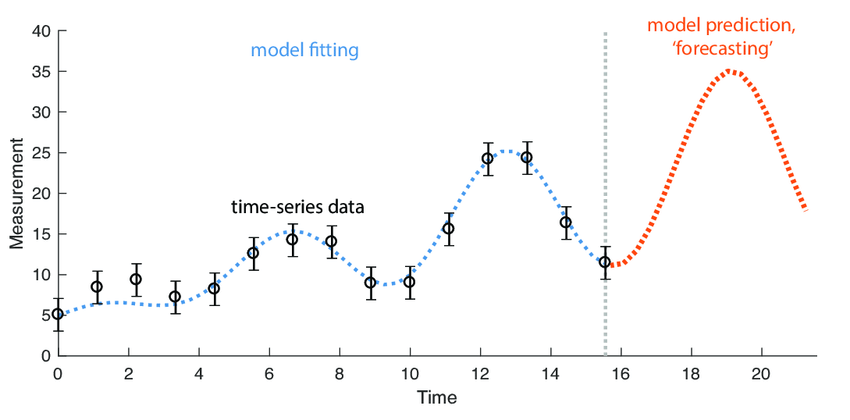
Time Series Forecasting: An Overview of Basic Concepts and Mechanisms

Time series forecasting is a statistical technique used to predict future values based on previously observed values, specifically in a sequence of data points collected over time. This method of analysis is widely employed across various fields, including finance, economics, weather forecasting, and inventory management.

What is a Time Series?

A time series is a collection of observations recorded sequentially over time. The observations are measured at evenly spaced intervals (seconds, minutes, etc.) or unevenly spaced interval. Time series data can be univariate (involving one variable) or multivariate (involving multiple variables).

Characteristics of Time Series Data

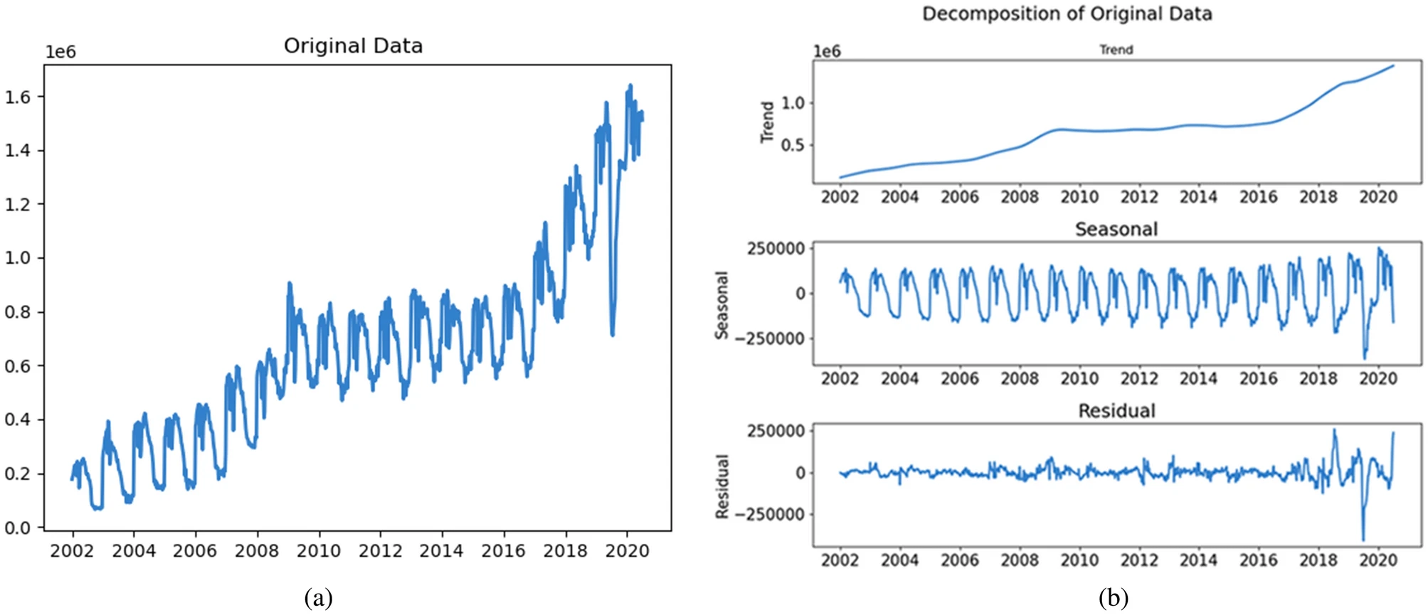
1. Trend: Refers to the long-term movement in the data. A trend can be upward, downward, or constant, and it reflects the overall direction as well as long-lasting patterns.
2. Seasonality: Refers to periodic fluctuations that can occur at regular intervals due to seasonal effects. For example, retail sales often increase during the holiday season every year.
3. Cyclic Patterns: Unlike seasonal fluctuations, cyclic patterns are irregular and do not have fixed periods. They are associated with economic or business cycles and may last from several months to years.
4. Residual (Noise): Random fluctuations in the data that can’t be attributed to trend or seasonality and typically arise from unpredictable influences.

Basic Concepts in Time Series Forecasting

1. Stationarity

Stationarity is a critical property of time series data. A stationary time series has statistical properties (mean, variance, autocorrelation) that do not change over time. Most time series forecasting models require the data to be stationary, as non-stationary data can lead to unreliable predictions.

Types of Stationarity:

• Strict Stationarity: The distribution of the time series is unchanged over time.
• Weak Stationarity: Only the first two moments (mean and variance) are constant over time.

If a time series is non-stationary, techniques such as differencing, transformation, or detrending can be applied to stabilize the series.

2. Autocorrelation

Autocorrelation measures the correlation between a time series and a lagged version of itself. It helps identify patterns and determines whether past values influence future values. The autocorrelation function (ACF) and the partial autocorrelation function (PACF) are essential tools for analyzing temporal dependencies in a time series.

Time Series Forecasting Methods

There are numerous methods available for time series forecasting. Some of the most commonly used methods include:

a. Naïve Method

The simplest form of forecasting methods relies on the assumption that future values will be similar to the most recent observed value. This approach is often used as a benchmark for evaluating more complex models.

b. Moving Average

The moving average method smooths out short-term fluctuations by averaging a specific number of past observations. There are two common types:

• Simple Moving Average (SMA): The average of a fixed number of past observations.
• Weighted Moving Average (WMA): Averages with weights assigned to different values, allowing more recent data to have a greater influence.

c. Exponential Smoothing

Exponential smoothing methods give more weight to recent observations, making them more responsive to changes in the data. The most common forms include:

• Simple Exponential Smoothing (SES): Best for data without trend or seasonality.
• Holt’s Linear Trend Model: Suitable for data exhibiting linear trends.
• Holt-Winters Seasonal Model: Designed for data with both trend and seasonality.

d. ARIMA (Autoregressive Integrated Moving Average)

ARIMA combines autoregression, differentiation, and moving average components.

• AR (Autoregressive) component: Relies on the dependency between an observation and a number of lagged observations.
• I (Integrated) component: Involves differencing the data to achieve stationarity.
• MA (Moving Average) component: Relates to the dependency between an observation and a residual error.

It is ideal for modeling non-stationary time series data and requires practitioners to identify the appropriate order of the AR and MA components. The model is denoted as ARIMA(p,d,q), where:

• p: order of the autoregressive part,
• d: degree of differencing needed for stationarity,
• q: order of the moving average part.

e. Seasonal Decomposition of Time Series (STL)

STL decomposes a time series into its seasonal, trend, and residual components, allowing for better understanding and modeling of each component separately. It is particularly useful for time series with strong seasonal effects.

f. Machine Learning Approaches

• Regression Models: Linear or nonlinear regression approaches can capture trends and seasonal effects in the time series data.
• Random Forest: An ensemble learning method that can capture non-linear relationships in the data and handle high dimensionality, making it suitable for complex time series.  
• Recurrent Neural Networks (RNNs): These neural networks (LSTMs, GRUs, etc) are designed to handle sequential data, making them suitable for time series. They have “memory” that allows them to remember past information and use it for future predictions.  
• Support Vector Regression (SVR): A powerful regression technique that can be adapted for time series forecasting by using past values as features.  
• Prophet: Developed by Facebook, this model is designed for time series with strong seasonality and holiday effects.It’s robust to missing data and outliers.

Evaluating Forecasting Performance

To assess the accuracy of forecasting models, various metrics are used, including:

• Mean Absolute Error (MAE): Average of absolute errors between forecasted and actual values.
• Mean Squared Error (MSE): Average of squared differences between forecasted and actual values. It penalizes larger errors more significantly.
• Root Mean Squared Error (RMSE): The square root of MSE, facilitating interpretation by reducing scale effects.
• Mean Absolute Percentage Error (MAPE): A percentage-based measure that is scale-invariant and provides a clear understanding of forecast accuracy.

Challenges in Time Series Forecasting

1. Non-stationarity: Many time series are non-stationary, meaning their statistical properties change over time. This condition complicates model selection and accuracy.
2. Seasonality Changes: Seasonal patterns may evolve, making it difficult to rely on past seasonal behavior.
3. Irregular Trends: Sudden shifts in trends, such as economic crises or natural disasters, can lead to significant forecasting errors.
4. Data Quality: Missing values, outliers, or noise in the data can significantly impair the accuracy of forecasts.
5. Model Overfitting: Complex models may capture noise instead of the actual underlying patterns, resulting in poor out-of-sample performance.

Applications of Time Series Forecasting

• Finance: Predicting stock prices, currency exchange rates, and credit risk assessments.
• Weather: Forecasting temperature, rainfall, and severe weather events.
• Economics: Analyzing economic indicators like GDP, consumer spending, and unemployment rates.
• Marketing: Estimating demand for products and planning promotional campaigns.
• Healthcare: Forecasting disease outbreaks and patient inflow in hospitals.
• Manufacturing: Inventory management and demand forecasting for optimal production planning.