Vision Transformers (ViT) have emerged as a groundbreaking architecture that has revolutionized how computers perceive and understand visual data. Introduced by researchers at Google Research in a seminal paper titled “An Image is Worth 16×16 Words: Transformers for Image Recognition at Scale” in 2020, ViTs have demonstrated the ability to outperform traditional convolutional neural networks (CNNs) on a variety of visual recognition tasks. This article aims to provide an extensive overview of Vision Transformers.
The Evolution of Vision Models
CNNs are structured to process images through convolutions, pooling layers, and non-linear activations. Over the years, they have proven effective for image classification, detection, and segmentation tasks.
However, the rise of transformers in NLP has sparked interest in applying these architectures to vision tasks. Introduced by Vaswani et al. in 2017 paper “Attention is All You Need”, the Transformer architecture utilizes self-attention mechanisms to weigh the significance of different parts of an input sequence dynamically. This capability allows Transformers to understand relationships that are far apart in the input data.
Vision Transformers (ViTs) adapt the Transformer architecture to process images. Instead of using convolutions to extract features, ViTs treat image patches as sequences, thus enabling the application of self-attention mechanisms to spatial data. The fundamental idea behind ViTs is to leverage the attention mechanism on flattened image segments, transforming image classification tasks.
An Overview of the ViT Architecture
Now that we’ve established the foundational concepts, let’s delve deeper into the architecture of Vision Transformers:
- Input Representation: An input image of dimensions \( H \times W \times C \) (Height, Width, Channels) is first resized to a dimension of \( H’ \times W’ \) (where \( H’ \) and \( W’ \) are downsampled sizes). The image is then sliced into non-overlapping patches of size \( P \times P \).
- Patch Embedding: Each \( P \times P \) patch is flattened into a vector of dimension \( P^2 \times C \). A linear layer projects it into a lower-dimensional space, creating patch embeddings.
- Positional Encoding: A positional encoding vector is added to each patch embedding to retain spatial context. This encoding can be learned or predefined (such as using sine and cosine functions).
- Self-Attention Mechanism: This is the core module. It allows each patch to aggregate information from all other patches, emphasizing the relationships across spatial areas.
- Calculation involves computing three matrices (Queries, Keys, and Values) from the patch embeddings. The self-attention score is derived as follows:
\[
\text{Attention}(Q, K, V) = \text{Softmax}\left(\frac{QK^T}{\sqrt{d_k}}\right)V
\]
Where \( d_k \) is the dimension of the key vector, ensuring numerical stability.
- Multi-head Self-Attention: ViTs deploy self-attention on the sequence of patch embeddings. This means that every patch can attend to every other patch, forming richer representations and relationships.
- Feed-Forward Network (FFN): After self-attention, the output is passed through a position-wise feed-forward network (typically two linear layers with a ReLU activation in between).
- Layer Normalization and Residual Connections: Each sub-layer in a ViT uses layer normalization and residual connections, improving training dynamics and enabling deeper architectures.
- Stacking Layers: Multiple attention layers can be stacked to create deep representation. This is similar to stacking convolutional layers in CNNs.
- Classification Head: For image classification, a special token (often referred to as [CLS]) is added to the sequence of embeddings at the beginning. After the final transformer block, the representation corresponding to this token is passed through a softmax layer for classification.
A Simple Example
To understand the ViT architecture, consider a simplified example of a 32×32 RGB image:
- Patch Size: Suppose we choose a patch size of \( 8 \times 8 \). The image can be divided into \( 16 \) patches (4 patches along the height and 4 patches along the width).
- Patch Flattening: Each \( 8 \times 8 \) patch is flattened into a vector of size \( 8^2 \times 3 = 192 \) (as there are 3 color channels).
- Creating Embedding: A linear layer transforms each patch’s flattened representation into a feature vector of size \( D \) (for instance, \( D = 128 \)).
- Positional Encoding: Positional encoding vectors are combined with patch embeddings. Assuming we use simple sine-cosine functions for positional encoding, we ensure that the positions of patches are retained.
- Self-Attention Application: Compute attention scores for all patches. For instance, patch \( A \) might pay attention more to patches \( B \) and \( C \) if they cover relevant contextual features.
- FFN Processing: The resulting embeddings pass through feed-forward networks, followed by residual connections and normalization.
- Classification: An additional [CLS] token learns the global representation, enabling image classification with a final softmax layer.
ViT Variants
Since the inception of the original ViT, several variants have been proposed to enhance its performance, including:
- DeiT (Data-efficient Image Transformers): Aimed at reducing the amount of training data needed by using techniques like knowledge distillation.
- Swin Transformer: Introduces a hierarchical architecture that allows for dense pixel representations and computes attention within local windows.
- CrossViT: Combines convolutional layers and attention mechanisms to leverage both local and global feature extraction.
Benefits of Vision Transformers
Vision Transformers present several advantages over traditional CNNs, notably:
- Scalability: ViTs can efficiently scale to larger datasets and more extensive model sizes, relying on the self-attention mechanism that enables capturing dependencies regardless of distance in the sequence of patches.
- Pre-training: Like their NLP counterparts, ViTs leverage large-scale unsupervised pre-training on vast image datasets (like ImageNet-21K). This pre-training approach can lead to significant performance improvements on downstream tasks.
- Reduced Inductive Bias: While CNNs impose strong inductive biases reflecting local patterns and spatial hierarchies, ViTs operate more flexibly, often generalizing better across various vision tasks, including those that do not conform to traditional visual patterns.
- Better Global Context Modeling: ViTs excel in capturing long-range relationships across an image, a problem that traditional CNNs struggle with without extensive architectural modifications.
- Transfer Learning: ViTs can transfer learned knowledge across different domains, as evidenced by their performance on various image classification benchmarks.
Challenges and Limitations
- Data-Hungry: ViTs often require vast amounts of data for training. In scenarios with limited labeled data, they may underperform compared to well-tuned CNNs.
- Computational Expense: The self-attention mechanism’s quadratic complexity may lead to increased computational requirements, especially for larger images or deeper architectures.
- Interpretability: Like other deep learning models, ViTs can be seen as black boxes, making interpretation of their decisions challenging. Understanding which patches influence specific predictions can be complex.
Applications of Vision Transformers
- Image Classification: ViTs have been widely used in image classification benchmarks, outperforming some traditional architectures and achieving state-of-the-art results.
- Object Detection: ViTs can be integrated into detection frameworks (like DETR) to enable effective object localization and classification.
- Image Segmentation: Vision Transformers can be adapted for segmentation tasks by using pixel-level predictions, allowing them to delineate object boundaries more accurately.
- Video Understanding: The same self-attention mechanism can be extended to process sequences of frames, aiding in motion detection, action recognition, and temporal coherence assessments.
- Medical Imaging: The capacity to model long-range correlations in data makes ViTs suitable candidates for processing medical images, such as MRI scans or X-rays, for diagnostic purposes.
The Future of Vision Transformers
- Reducing Computational Load: Exploring efficient attention mechanisms, such as linear or sparse attention, to alleviate the quadratic complexity of standard transformers.
- Hybrid Architectures: Combining the strengths of CNNs and ViTs to create hybrid models that leverage both local feature extraction and global context modeling.
- Improved Training Techniques: Investigating better training schemes, such as few-shot learning or self-supervised techniques, to enable robust performance with smaller datasets.
- Broader Applications: Extending ViTs to multi-modal tasks, incorporating both vision and language, to enhance tasks like image captioning, visual question answering, and interactive AI systems.
- Enhanced Interpretability: Improving interpretability through model explanations, saliency mapping, and other techniques will be crucial to building trust in Vision Transformers, especially in sensitive industries.
Conclusion
Vision Transformers represent a paradigm shift in the field of computer vision, redefining the standards of image recognition and visual understanding. By drawing from the successful self-attention mechanisms of NLP, ViTs have showcased incredible prowess in various tasks. Although challenges remain in areas like data efficiency and computational intensity, ongoing research is making strides toward enhancing their utility and accessibility.
Q: How to compute the number of tokens for a ViT?

Silpa brings 5 years of experience in working on diverse ML projects, specializing in designing end-to-end ML systems tailored for real-time applications. Her background in statistics (Bachelor of Technology) provides a strong foundation for her work in the field. Silpa is also the driving force behind the development of the content you find on this site.
Subscribe to our newsletter!