Variational Autoencoders (VAEs): Intuition, Math, and Practical Implementation

Imagine you are trying to teach a computer to paint.

A classic autoencoder is a skilled copier: it learns an encoder (compress) and a decoder (decompress) and can reconstruct inputs well. However, its latent space often ends up shaped like disconnected islands. Many random latent points decode to nonsense, because nothing forces the encoder to organize latent space globally.

A variational autoencoder (VAE) turns that latent space into a navigable map. Instead of mapping each input to a single point, it maps each input $x$ to a distribution over latent codes $z$, and it nudges those distributions toward a simple prior (usually a standard normal). This is what makes VAEs generative: sampling $z \sim \mathcal{N}(0, I)$ has a reasonable chance of decoding into a plausible sample.

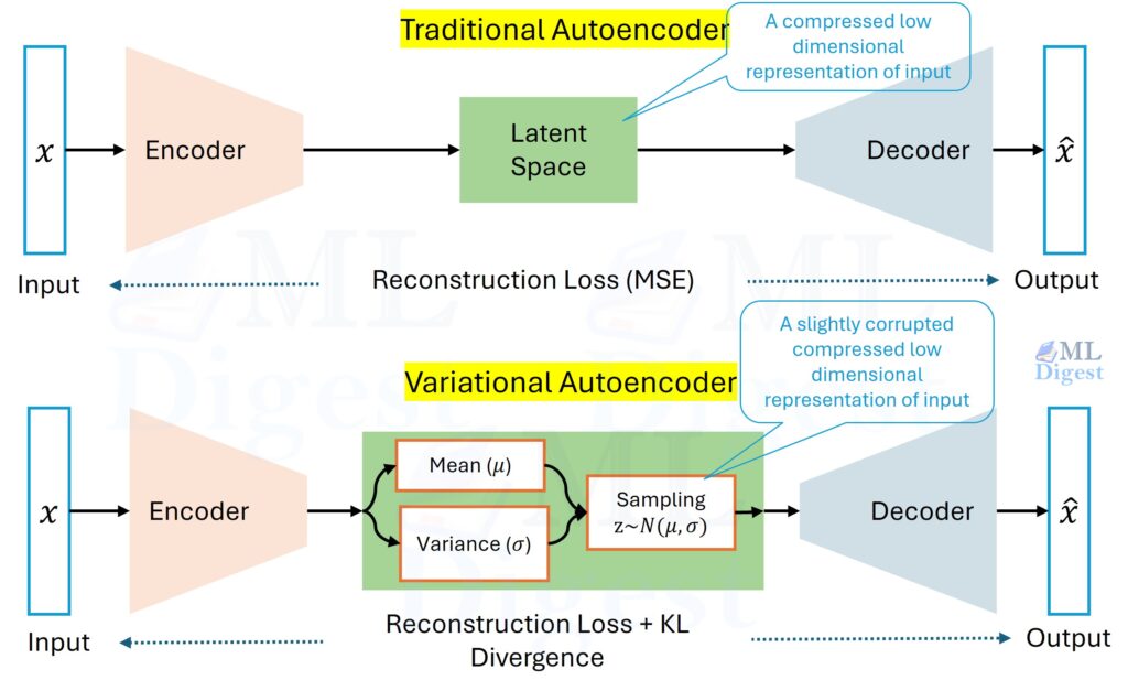
(Figure: The difference between standard autoencoders and variational autoencoders. In a standard autoencoder, each input maps to a discrete point in latent space, leading to gaps and unstructured regions. In a VAE, inputs are mapped to distributions that overlap and fill the space, creating a continuous manifold where every point decodes to something meaningful.)

If you move slightly in latent space, the decoded output typically changes smoothly. In a mental picture, imagine a “cat region” in latent space: a small step changes pose or lighting rather than turning the cat into noise.

The Big Idea: Standard autoencoders learn discrete points. VAEs learn probability distributions. This difference allows VAEs to dream new data.

Why VAEs matter

VAEs are a foundational generative modeling approach. While diffusion models (like Stable Diffusion and DALL-E) have taken the spotlight for high-fidelity images, VAEs remain important because:

1. They are fast at sampling: Unlike diffusion models which require many steps, VAEs generate data in a single forward pass.
2. They are probabilistic: They optimize a well-defined mathematical objective (the ELBO).
3. Smooth Latent Spaces: They are excellent for tasks like interpolation (morphing one image into another) and manipulating features (adding “smile” to a face vector).
4. They are the Engine of Latent Diffusion: Stable Diffusion is a latent diffusion model, and the “latent” space is produced by a VAE. The VAE compresses images into a compact representation where diffusion is performed. Without this compression, diffusion on full-resolution pixels is far more expensive.

Common applications:

• Data generation and augmentation (images, features, audio embeddings)
• Representation learning (compact continuous embeddings)
• Anomaly detection (high reconstruction error, or low likelihood-based scores)
• Compression with uncertainty (stochastic latent codes)
• Conditional generation (cVAE for class-conditional or attribute-conditional synthesis)

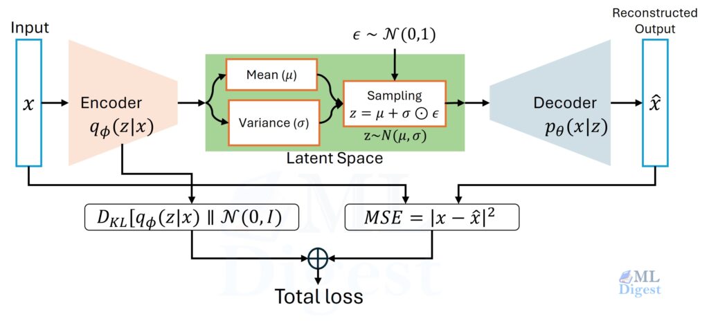
The Mechanics: Mapping Inputs to Distributions

To understand this “fuzzy map” idea, the key change is simple: the bottleneck is not a single vector, but a distribution.

You can visualize a VAE as two maps between spaces:

1. Encoder: takes an input $x$ and outputs parameters of a distribution over latent variables $z$.
2. Decoder: takes a latent sample $z$ and outputs parameters of a distribution over $x$.

1. The Probabilistic Encoder

In a standard autoencoder, the encoder is a function $z = f(x)$. It outputs a single vector.
In a VAE, the encoder doesn’t output a coordinate; it outputs parameters of a probability distribution. We typically assume this distribution is Gaussian (a bell curve), which is defined by two things: a center ($\mu$) and a spread ($\sigma$).

So, the encoder becomes “two-headed”:

1. $\mu_\phi(x)$ (mean): the center. Intuitively: “the best guess for where this example lives.”
2. $\log \sigma^2_\phi(x)$ (log-variance): the uncertainty/spread. Intuitively: “how wide is the region?”

Mathematically, this defines our approximate posterior distribution, $q_\phi(z\mid x)$:
$$
q_\phi(z\mid x) = \mathcal{N}\big(z;\, \mu_\phi(x),\, \mathrm{diag}(\sigma^2_\phi(x))\big)
$$

Note the roles of the symbols:

• $\theta$: decoder (generative) parameters
• $\phi$: encoder (inference) parameters
• $q_\phi(z\mid x)$: approximate posterior (“where does the encoder place $x$ in latent space?”)
• $p(z)$: prior (“where will I sample from at generation time?”)

The true posterior $p_\theta(z\mid x)$ is typically intractable because it depends on the marginal likelihood $p_\theta(x)$.
So we approximate it with $q_\phi(z\mid x)$, learned via amortized inference.

2. The Probabilistic Decoder (Generative Model)

The decoder takes a sample $z$ and reconstructs the data by defining a conditional distribution:
$$
p_\theta(x\mid z)
$$
This is the generative model. Ideally, if you sample $z$ from the “cat region” implied by the encoder, the decoder should produce an image that still looks like a cat.

We specify a prior and a likelihood:

• Prior: $p(z) = \mathcal{N}(0, I)$ (most common)
• Likelihood: $p_\theta(x\mid z)$ parameterized by a neural network

The Objective: ELBO (Evidence Lower Bound)

Training a VAE is a balancing act between two goals: (1) reconstruct the input well and (2) keep the latent distributions compatible with the prior so that sampling works. This trade-off is captured by the Evidence Lower Bound (ELBO).

The quantity you would like to maximize is the marginal log-likelihood:
$$
\log p_\theta(x),\quad \text{where}\quad p_\theta(x)=\int p_\theta(x\mid z)p(z)\,dz.
$$
The integral is typically intractable for neural decoders.

Variational inference introduces an approximate posterior $q_\phi(z\mid x)$ and yields a lower bound on $\log p_\theta(x)$ (the ELBO):
$$
\mathrm{ELBO}(x)=\underbrace{\mathbb{E}_{q_\phi(z\mid x)}[\log p_\theta(x\mid z)]}_{\text{Reconstruction term}}-\underbrace{\mathrm{KL}\big(q_\phi(z\mid x)\,|\,p(z)\big)}_{\text{Regularization term}}.
$$

Reconstruction Loss (“Be Accurate”)

• Goal: Make the decoded output look exactly like the input.
• Intuition: This term tries to make the distributions $\mu(x)$ as specific and narrow as possible. Ideally, the encoder would shrink the variance $\sigma$ to zero so the decoder knows exactly what to draw.
• Consequence if unchecked: The model becomes a standard autoencoder. It learns to copy data perfectly but fails to generate anything new because the latent space becomes a set of disconnected points.

Regularization (KL Divergence) (“Be Organized”)

• Goal: Force the latent distribution $q_\phi(z|x)$ to look like the standard normal prior $p(z) = \mathcal{N}(0, I)$.
• Intuition: This term is the “packer.” It penalizes encoder posteriors that drift too far from the prior distribution.
• It prevents the encoder from “cheating” by making variances zero (which would turn it back into a point-estimate autoencoder).
• It pushes all the little distributions toward the center $(0,0)$ and forces them to have unit variance, ensuring the space is dense and sampleable.
• Consequence if unchecked: Total chaos. If this term dominates (e.g., if the weight $\beta$ is too high), the encoder ignores the input image and just outputs a generic Gaussian blob for everything. This is called Posterior Collapse. The decoder receives pure noise and generates the “average” image (often a blurry gray mess).

The Sweet Spot

The magic happens in the balance. The Reconstruction loss pulls the distributions apart (to distinguish cats from dogs), while the Regularization term pulls them together (so they overlap and form a smooth manifold). This is the central trade-off in VAEs: fidelity versus a sampleable latent distribution.

Two clarifications that prevent common confusion:

1. The “reconstruction loss” is (up to constants) the negative log-likelihood under the chosen likelihood $p_\theta(x\mid z)$. MSE and BCE are modeling choices because they correspond to different likelihood assumptions.
2. The KL term makes sampling from the prior meaningful, but it does not guarantee high-quality samples early in training. Sample quality often lags reconstruction quality.

In most implementations, you minimize the negative ELBO (a loss):
$$
\mathcal{L}(x)= -\mathbb{E}_{q_\phi(z\mid x)}[\log p_\theta(x\mid z)] + \beta\,\mathrm{KL}\big(q_\phi(z\mid x)\,|\,p(z)\big).
$$
The hyperparameter $\beta$ is $1$ for the standard VAE. It is adjusted in $\beta$-VAE or changed over time in KL warm-up schedules.

A Useful Identity (optional, but clarifying)

The ELBO is not a heuristic. It satisfies:
$$
\log p_\theta(x) = \mathrm{ELBO}(x) + \mathrm{KL}\big(q_\phi(z\mid x)\,|\,p_\theta(z\mid x)\big)
$$
Since KL is nonnegative, maximizing the ELBO simultaneously increases a lower bound on $\log p_\theta(x)$ and pushes $q_\phi(z\mid x)$ toward the true posterior.

This identity is also a useful debugging lens: it separates “how tight the bound is” from “how good reconstructions look.” A model can reconstruct reasonably well while still generating poorly if the learned posteriors are not well aligned with the prior used at sampling time.

Why the KL Has a Closed Form (Diagonal Gaussian Case)

If the approximate posterior is diagonal Gaussian and the prior is standard normal, the KL divergence has a closed-form expression. This is one reason the “Gaussian VAE” is so practical.

If $q_\phi(z\mid x)=\mathcal{N}(\mu, \mathrm{diag}(\sigma^2))$ and $p(z)=\mathcal{N}(0, I)$, then:

$$
\mathrm{KL}(q|p) = \frac{1}{2}\sum_{j=1}^d\Big(\mu_j^2 + \sigma_j^2 – \log\sigma_j^2 – 1\Big)
$$

In practice: Most implementations predict $\log\sigma^2$ for numerical stability, and compute this expression without ever explicitly forming a covariance matrix. Common questions

The Reparameterization Trick (How Gradients Flow)

How to backpropagate through randomness

We hit a major roadblock when training. The network needs to sample $z$ from the distribution defined by $(\mu, \sigma)$. Naively sampling $z \sim \mathcal{N}(\mu, \sigma^2)$ breaks backpropagation, because sampling is not differentiable.

Sampling is a stochastic process: it is like rolling dice. You cannot compute a gradient through a dice roll. If gradients cannot pass through the sampling step, the encoder cannot learn.

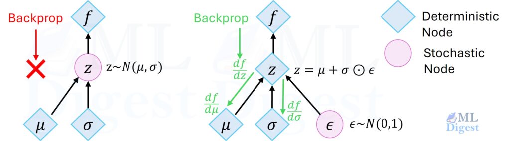
The solution is the reparameterization trick. Rewrite sampling so that randomness is moved “outside” the network: treat it as an external noise input.

1. Sample noise $\epsilon \sim \mathcal{N}(0, I)$ independently (no gradients needed here).
2. Compute $z$ as a deterministic function of $\mu$, $\sigma$, and $\epsilon$:
   $$
   z = \mu_\phi(x) + \sigma_\phi(x) \odot \epsilon
   $$

Now, $z$ is just a linear transformation (differentiable function) of $\mu$ and $\sigma$. The randomness is shunted to $\epsilon$, which is a leaf node in the computational graph. Gradients can flow freely through $\mu$ and $\sigma$ because they are now just involved in standard addition and multiplication.

Choosing the Likelihood: Match $p_\theta(x\mid z)$ to the Data

Do not optimize the wrong objective.

This is one of the most common sources of silently bad VAEs. Training can look stable while the model optimizes a likelihood that does not match the data, which changes what the reconstruction term means.

1. Continuous data (sensors, embeddings, standardized features):
   Use a Gaussian likelihood. A common simplification is to let the decoder output a mean $\hat{x}$ and use an MSE-like reconstruction term (equivalent to a Gaussian with fixed variance, up to constants).
2. Binary or near-binary data (MNIST-style pipelines in $[0,1]$):
   Use a Bernoulli likelihood. The decoder outputs logits and the reconstruction term becomes binary cross-entropy.

Practical note: for images, scaling to $[0,1]$ and using BCE can work well, but it is a modeling choice. If pixels are not truly Bernoulli, a Gaussian or discretized-logistic likelihood can behave better.

Another practical note: with continuous images in $[0,1]$, BCE often pushes predictions toward extremes (close to 0 or 1). That can be desirable for binarized data, but it may be overconfident for natural images.

A quick rule of thumb

• If $x$ is best thought of as continuous (normalized sensor features, embeddings), start with a Gaussian likelihood.
• If $x$ is genuinely binary, or you explicitly use Bernoulli as a pragmatic approximation (for example, some MNIST-style pipelines), use a Bernoulli likelihood.

Implementation Steps (End-to-End)

1. Define an encoder network producing $(\mu, \log\sigma^2)$
2. Sample $z$ via reparameterization
3. Define a decoder network producing distribution parameters for $x$
4. Compute the loss
   • Reconstruction term (negative log-likelihood)
   • KL divergence to the prior
5. Train with stochastic gradient descent (often Adam)
6. Generate samples by drawing $z \sim \mathcal{N}(0, I)$ and decoding

Informally, training mostly lives in steps 4 and 5: you repeatedly (a) sample a latent code using the encoder distribution and (b) update encoder and decoder to increase the ELBO.

One “sanity diagram” worth keeping in mind:

• Training path: $x \rightarrow q_\phi(z\mid x) \rightarrow z \rightarrow p_\theta(x\mid z)$
• Generation path: $z \sim p(z) \rightarrow p_\theta(x\mid z)$

Many VAE issues are failures to make these two paths compatible.

A minimal PyTorch VAE (runnable)

This is a small, fully-contained VAE suitable for vector inputs (for example, flattened MNIST-sized inputs). It includes two reconstruction options:

• Bernoulli likelihood via BCE (works when inputs are in $[0,1]$)
• Gaussian likelihood via MSE (common for continuous features)

import math
from dataclasses import dataclass

import torch
import torch.nn as nn
import torch.nn.functional as F


class MLPEncoder(nn.Module):
    def __init__(self, input_dim: int, hidden_dim: int, latent_dim: int):
        super().__init__()
        self.net = nn.Sequential(
            nn.Linear(input_dim, hidden_dim),
            nn.ReLU(),
            nn.Linear(hidden_dim, hidden_dim),
            nn.ReLU(),
        )
        self.mu = nn.Linear(hidden_dim, latent_dim)
        self.logvar = nn.Linear(hidden_dim, latent_dim)

    def forward(self, x: torch.Tensor) -> tuple[torch.Tensor, torch.Tensor]:
        h = self.net(x)
        return self.mu(h), self.logvar(h)


class MLPDecoder(nn.Module):
    def __init__(self, latent_dim: int, hidden_dim: int, output_dim: int):
        super().__init__()
        self.net = nn.Sequential(
            nn.Linear(latent_dim, hidden_dim),
            nn.ReLU(),
            nn.Linear(hidden_dim, hidden_dim),
            nn.ReLU(),
            nn.Linear(hidden_dim, output_dim),
        )

    def forward(self, z: torch.Tensor) -> torch.Tensor:
        # Return logits for Bernoulli likelihood
        return self.net(z)


class VAE(nn.Module):
    def __init__(self, input_dim: int, hidden_dim: int, latent_dim: int):
        super().__init__()
        self.encoder = MLPEncoder(input_dim, hidden_dim, latent_dim)
        self.decoder = MLPDecoder(latent_dim, hidden_dim, input_dim)

    @staticmethod
    def reparameterize(mu: torch.Tensor, logvar: torch.Tensor) -> torch.Tensor:
        # logvar = log(sigma^2)
        std = torch.exp(0.5 * logvar)
        eps = torch.randn_like(std)
        return mu + std * eps

    @staticmethod
    def kl_divergence(mu: torch.Tensor, logvar: torch.Tensor) -> torch.Tensor:
        # KL(N(mu, sigma^2) || N(0,1)) summed over latent dims
        # 0.5 * sum(mu^2 + sigma^2 - log(sigma^2) - 1)
        return 0.5 * torch.sum(mu.pow(2) + logvar.exp() - logvar - 1.0, dim=1)

    def forward(self, x: torch.Tensor) -> dict[str, torch.Tensor]:
        mu, logvar = self.encoder(x)
        z = self.reparameterize(mu, logvar)
        logits = self.decoder(z)
        return {"logits": logits, "mu": mu, "logvar": logvar, "z": z}


@dataclass
class LossOutput:
    loss: torch.Tensor
    recon: torch.Tensor
    kl: torch.Tensor


def vae_loss_bce(
    x: torch.Tensor,
    logits: torch.Tensor,
    mu: torch.Tensor,
    logvar: torch.Tensor,
    beta: float = 1.0,
) -> LossOutput:
    # Reconstruction term: negative log-likelihood under Bernoulli
    # BCEWithLogits computes per-element BCE; sum over feature dims.
    recon = F.binary_cross_entropy_with_logits(logits, x, reduction="none").sum(dim=1)
    kl = VAE.kl_divergence(mu, logvar)
    loss = (recon + beta * kl).mean()
    return LossOutput(loss=loss, recon=recon.mean(), kl=kl.mean())


def vae_loss_mse(
    x: torch.Tensor,
    x_hat: torch.Tensor,
    mu: torch.Tensor,
    logvar: torch.Tensor,
    beta: float = 1.0,
) -> LossOutput:
    # Gaussian likelihood with fixed variance corresponds to an MSE-like term
    # (ignoring constants). Sum over feature dimensions for a per-example NLL.
    recon = F.mse_loss(x_hat, x, reduction="none").sum(dim=1)
    kl = VAE.kl_divergence(mu, logvar)
    loss = (recon + beta * kl).mean()
    return LossOutput(loss=loss, recon=recon.mean(), kl=kl.mean())


def train_one_epoch(
    model: nn.Module,
    optimizer: torch.optim.Optimizer,
    data_loader,
    device: torch.device,
    beta: float = 1.0,
) -> dict[str, float]:
    model.train()
    total_loss = 0.0
    total_recon = 0.0
    total_kl = 0.0
    n = 0

    for x, *_ in data_loader:
        x = x.to(device)
        x = x.view(x.size(0), -1)

        out = model(x)
        loss_out = vae_loss_bce(x, out["logits"], out["mu"], out["logvar"], beta=beta)

        optimizer.zero_grad(set_to_none=True)
        loss_out.loss.backward()
        optimizer.step()

        batch_size = x.size(0)
        total_loss += loss_out.loss.item() * batch_size
        total_recon += loss_out.recon.item() * batch_size
        total_kl += loss_out.kl.item() * batch_size
        n += batch_size

    return {
        "loss": total_loss / n,
        "recon": total_recon / n,
        "kl": total_kl / n,
    }


@torch.no_grad()
def sample(model: VAE, num_samples: int, device: torch.device) -> torch.Tensor:
    model.eval()
    latent_dim = model.encoder.mu.out_features
    z = torch.randn(num_samples, latent_dim, device=device)
    logits = model.decoder(z)
    probs = torch.sigmoid(logits)
    return probs

import math
from dataclasses import dataclass

import torch
import torch.nn as nn
import torch.nn.functional as F


class MLPEncoder(nn.Module):
    def __init__(self, input_dim: int, hidden_dim: int, latent_dim: int):
        super().__init__()
        self.net = nn.Sequential(
            nn.Linear(input_dim, hidden_dim),
            nn.ReLU(),
            nn.Linear(hidden_dim, hidden_dim),
            nn.ReLU(),
        )
        self.mu = nn.Linear(hidden_dim, latent_dim)
        self.logvar = nn.Linear(hidden_dim, latent_dim)

    def forward(self, x: torch.Tensor) -> tuple[torch.Tensor, torch.Tensor]:
        h = self.net(x)
        return self.mu(h), self.logvar(h)


class MLPDecoder(nn.Module):
    def __init__(self, latent_dim: int, hidden_dim: int, output_dim: int):
        super().__init__()
        self.net = nn.Sequential(
            nn.Linear(latent_dim, hidden_dim),
            nn.ReLU(),
            nn.Linear(hidden_dim, hidden_dim),
            nn.ReLU(),
            nn.Linear(hidden_dim, output_dim),
        )

    def forward(self, z: torch.Tensor) -> torch.Tensor:
        # Return logits for Bernoulli likelihood
        return self.net(z)


class VAE(nn.Module):
    def __init__(self, input_dim: int, hidden_dim: int, latent_dim: int):
        super().__init__()
        self.encoder = MLPEncoder(input_dim, hidden_dim, latent_dim)
        self.decoder = MLPDecoder(latent_dim, hidden_dim, input_dim)

    @staticmethod
    def reparameterize(mu: torch.Tensor, logvar: torch.Tensor) -> torch.Tensor:
        # logvar = log(sigma^2)
        std = torch.exp(0.5 * logvar)
        eps = torch.randn_like(std)
        return mu + std * eps

    @staticmethod
    def kl_divergence(mu: torch.Tensor, logvar: torch.Tensor) -> torch.Tensor:
        # KL(N(mu, sigma^2) || N(0,1)) summed over latent dims
        # 0.5 * sum(mu^2 + sigma^2 - log(sigma^2) - 1)
        return 0.5 * torch.sum(mu.pow(2) + logvar.exp() - logvar - 1.0, dim=1)

    def forward(self, x: torch.Tensor) -> dict[str, torch.Tensor]:
        mu, logvar = self.encoder(x)
        z = self.reparameterize(mu, logvar)
        logits = self.decoder(z)
        return {"logits": logits, "mu": mu, "logvar": logvar, "z": z}


@dataclass
class LossOutput:
    loss: torch.Tensor
    recon: torch.Tensor
    kl: torch.Tensor


def vae_loss_bce(
    x: torch.Tensor,
    logits: torch.Tensor,
    mu: torch.Tensor,
    logvar: torch.Tensor,
    beta: float = 1.0,
) -> LossOutput:
    # Reconstruction term: negative log-likelihood under Bernoulli
    # BCEWithLogits computes per-element BCE; sum over feature dims.
    recon = F.binary_cross_entropy_with_logits(logits, x, reduction="none").sum(dim=1)
    kl = VAE.kl_divergence(mu, logvar)
    loss = (recon + beta * kl).mean()
    return LossOutput(loss=loss, recon=recon.mean(), kl=kl.mean())


def vae_loss_mse(
    x: torch.Tensor,
    x_hat: torch.Tensor,
    mu: torch.Tensor,
    logvar: torch.Tensor,
    beta: float = 1.0,
) -> LossOutput:
    # Gaussian likelihood with fixed variance corresponds to an MSE-like term
    # (ignoring constants). Sum over feature dimensions for a per-example NLL.
    recon = F.mse_loss(x_hat, x, reduction="none").sum(dim=1)
    kl = VAE.kl_divergence(mu, logvar)
    loss = (recon + beta * kl).mean()
    return LossOutput(loss=loss, recon=recon.mean(), kl=kl.mean())


def train_one_epoch(
    model: nn.Module,
    optimizer: torch.optim.Optimizer,
    data_loader,
    device: torch.device,
    beta: float = 1.0,
) -> dict[str, float]:
    model.train()
    total_loss = 0.0
    total_recon = 0.0
    total_kl = 0.0
    n = 0

    for x, *_ in data_loader:
        x = x.to(device)
        x = x.view(x.size(0), -1)

        out = model(x)
        loss_out = vae_loss_bce(x, out["logits"], out["mu"], out["logvar"], beta=beta)

        optimizer.zero_grad(set_to_none=True)
        loss_out.loss.backward()
        optimizer.step()

        batch_size = x.size(0)
        total_loss += loss_out.loss.item() * batch_size
        total_recon += loss_out.recon.item() * batch_size
        total_kl += loss_out.kl.item() * batch_size
        n += batch_size

    return {
        "loss": total_loss / n,
        "recon": total_recon / n,
        "kl": total_kl / n,
    }


@torch.no_grad()
def sample(model: VAE, num_samples: int, device: torch.device) -> torch.Tensor:
    model.eval()
    latent_dim = model.encoder.mu.out_features
    z = torch.randn(num_samples, latent_dim, device=device)
    logits = model.decoder(z)
    probs = torch.sigmoid(logits)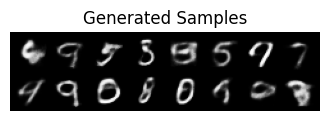
    return probs

How to use this with MNIST (minimal runnable sketch)

The model above expects a tensor of shape (batch, input_dim). For MNIST, input_dim=28*28=784.

Below is a minimal sketch that trains for a few epochs and samples digits. It is intentionally small and easy to modify.

import torch
from torch.utils.data import DataLoader
from torchvision import datasets, transforms
import matplotlib.pyplot as plt
import torchvision.utils as vutils

def main():
    device = torch.device("cuda" if torch.cuda.is_available() else "cpu")

    transform = transforms.Compose([transforms.ToTensor()])
    ds = datasets.MNIST(root="./data", train=True, download=True, transform=transform)
    loader = DataLoader(ds, batch_size=128, shuffle=True, num_workers=2, pin_memory=True)

    model = VAE(input_dim=28 * 28, hidden_dim=512, latent_dim=16).to(device)
    opt = torch.optim.Adam(model.parameters(), lr=1e-3)

    for epoch in range(5):
        metrics = train_one_epoch(model, opt, loader, device=device, beta=1.0)
        print(f"epoch={epoch} loss={metrics['loss']:.2f} recon={metrics['recon']:.2f} kl={metrics['kl']:.2f}")

    samples = sample(model, num_samples=16, device=device)
    samples = samples.view(-1, 1, 28, 28).cpu()
    print("sample batch:", samples.shape)

    # Visualize the generated samples
    plt.figure(figsize=(4, 4))
    plt.axis("off")
    plt.title("Generated Samples")
    plt.imshow(vutils.make_grid(samples, padding=2, normalize=True).permute(1, 2, 0))
    plt.show()


if __name__ == "__main__":
    main()

import torch
from torch.utils.data import DataLoader
from torchvision import datasets, transforms
import matplotlib.pyplot as plt
import torchvision.utils as vutils

def main():
    device = torch.device("cuda" if torch.cuda.is_available() else "cpu")

    transform = transforms.Compose([transforms.ToTensor()])
    ds = datasets.MNIST(root="./data", train=True, download=True, transform=transform)
    loader = DataLoader(ds, batch_size=128, shuffle=True, num_workers=2, pin_memory=True)

    model = VAE(input_dim=28 * 28, hidden_dim=512, latent_dim=16).to(device)
    opt = torch.optim.Adam(model.parameters(), lr=1e-3)

    for epoch in range(5):
        metrics = train_one_epoch(model, opt, loader, device=device, beta=1.0)
        print(f"epoch={epoch} loss={metrics['loss']:.2f} recon={metrics['recon']:.2f} kl={metrics['kl']:.2f}")

    samples = sample(model, num_samples=16, device=device)
    samples = samples.view(-1, 1, 28, 28).cpu()
    print("sample batch:", samples.shape)

    # Visualize the generated samples
    plt.figure(figsize=(4, 4))
    plt.axis("off")
    plt.title("Generated Samples")
    plt.imshow(vutils.make_grid(samples, padding=2, normalize=True).permute(1, 2, 0))
    plt.show()


if __name__ == "__main__":
    main()

If you switch to Gaussian reconstruction, replace the decoder output and loss accordingly:

• interpret the decoder output as $\hat{x}$ (a mean)
• use vae_loss_mse(x, x_hat, mu, logvar, beta=...)

A Practitioner’s Guide to Training VAEs

Training VAEs can be finicky. The loss is a delicate balance, and it is easy to fall into suboptimal states where the model effectively ignores latent space.

1. The Silent Failure: Posterior Collapse

The Symptom: KL divergence drops to nearly $0$, reconstruction improves, but samples look poor or nearly identical. Latent traversals have little effect.
The Reality: The decoder can become so strong that it ignores $z$ entirely. It behaves like an unconditional model (learning an average) rather than using $z$ as an information channel.
The Fixes:

• KL Annealing: Start with $\beta=0$ (pure reconstruction) and linearly ramp it up to $\beta=1$ over the first few epochs. This lets the encoder establish meaningful clusters before the regularization constraint tightens.
• Free Bits (KL Thresholding): Modify the loss to allow a small amount of KL divergence (e.g., 0.5 nats) without penalty. This prevents the optimizer from crushing the variance to the prior immediately.
• Weaken the Decoder: If you use a powerful autoregressive decoder (like an LSTM or Transformer), it may not need $z$ to predict pixels. Using a simpler decoder can force the model to rely on the content of $z$.

2. Disentanglement with $\beta$-VAE

The standard VAE ($\beta=1$) balances reconstruction and sampling.

• $\beta > 1$: Forces stronger independence between latent factors. This often aligns latent dimensions with semantic concepts (e.g., one dimension controls “smile,” another “rotation”), but at the cost of blurrier reconstructions.
• $\beta < 1$: Prioritizes reconstruction quality over structured latent space.

3. Evaluation Checklist (How to Know if it Works)

Accuracy numbers (MSE/BCE) are insufficient because they can favor safe, blurry averages.

1. Visual Inspection: Sample from the prior $z \sim \mathcal{N}(0, I)$. Do the images look valid?
2. Interpolation: Pick two real images, encode them into $z_1$ and $z_2$, and decode points along the line between them. A good VAE shows a smooth morphing transition.
3. Active Units: Measure how much each latent dimension varies with $x$ (for example, by tracking the variance of $\mu_\phi(x)$ over the dataset). Dimensions that barely move with $x$ are effectively unused.

4. Implementation Sanity Checks

• Log-Variance: Always predict logvar, not var or std, to avoid negative numbers and numerical instability.
• Data Range:
  • If using BCE Loss, your data must be in $[0, 1]$.
  • If using MSE Loss, your data is usually normalized (e.g., mean 0, std 1), and your decoder (typically) shouldn’t have a sigmoid at the end.
  • Mismatched loss and data range is the #1 cause of silent failure.

5. KL Explosion / NaNs

If you see NaNs in loss or gradients, it is often due to numerical instability in the variance computation.

• Clamp log-variance: Limit logvar to a reasonable range (e.g., [-10, 10]) during training.
• Reduce Learning Rate: A high learning rate can cause large updates that destabilize variance.
• Check Mixed Precision: If using mixed precision training, ensure that variance computations are stable.

Best practices (a checklist)

• Start simple: MLP VAE on vectors before convolutional VAE on images.
• Log recon and KL every epoch/step.
• Use KL warm-up for most non-trivial problems.
• Choose likelihood carefully (Bernoulli vs Gaussian).
• Compare against baselines: deterministic autoencoder and PCA.
• Inspect latent traversals: they reveal collapse quickly.
• Tune latent dimension: too small hurts recon; too large may collapse without proper regularization.

One more practical check: verify that you are consistent about whether reconstruction is summed over features or averaged. This choice changes the effective weighting between reconstruction and KL, which can otherwise look like a “mysterious” hyperparameter issue.

Variants worth knowing

Final Takeaways

• Intuition: Do not think of VAEs as file compressors. Think of them as map-makers: they learn a smooth latent space where nearby points decode to meaningfully related outputs.
• The Objective: Training maximizes the ELBO: a reconstruction expectation minus a KL regularizer to the prior.
• The Mechanics: The reparameterization trick rewrites sampling so gradients can flow.
• Practice: Most training issues reduce to (a) likelihood mismatch, (b) a misbalanced KL weight, or (c) posterior collapse.

If you remember one debugging mantra: check that your likelihood matches your data, and log reconstruction and KL separately.