With the advances of deep learning come challenges, most notably the issue of overfitting. Overfitting occurs when a model learns not only the underlying patterns in the training data but also the noise, leading to poor generalization on unseen data. Thus, regularization techniques have become indispensable tools for practitioners seeking to improve model robustness and performance.
Regularization methods work by introducing constraints or additional information into the learning process. The goal is to reduce the model’s capacity to memorize and to encourage it to learn more robust features.
In this article, we will explore various regularization techniques employed in neural networks. We will categorize these techniques into several key groups: L1 and L2 regularization, Dropout, Early Stopping, Batch Normalization, Data Augmentation, and more advanced methods such as Mixup, Cutout, and adversarial training.
Understanding Overfitting
A model is considered overfit when it captures the noise in the training data rather than the underlying patterns. This behavior typically arises in scenarios where the model complexity exceeds the complexity of the underlying data distribution, thus yielding a low training error but a high validation error.
Key indicators of overfitting include:
- High accuracy on training datasets but significantly lower accuracy on validation or test datasets.
- A large gap between training and validation loss.
The Bias-Variance Tradeoff
Regularization techniques often pivot on the bias-variance tradeoff. Bias refers to error due to simplifying assumptions in the learning algorithm, while variance reflects sensitivity to fluctuations in the training data. Striking the right balance between bias and variance is crucial for building models that generalize well.
Regularization can be viewed as a set of techniques applied during model training to discourage learning a model that is too complex, thereby enhancing generalization capabilities.
Common Regularization Techniques
1. L1 and L2 Regularization
L1 Regularization (Lasso Regularization): Adds an L1 penalty to the loss function, which is the sum of the absolute values of the model parameters. The L1 regularization term can promote sparsity, effectively driving some weights to zero.
Mathematically, the total loss function can be expressed as:
\[ \text{Loss} = L(y, \hat{y}) + \lambda \sum_{i=1}^{n} |w_i| \]
where \( L \) is the original loss function, \( y \) is the true value, \( \hat{y} \) is the predicted value, \( n \) is the number of weights, \( w_i \) is the weight, and \( \lambda \) is a hyperparameter that controls the strength of the regularization.
L2 Regularization (Ridge Regularization or Weight Decay): Incorporates an L2 penalty, which is the sum of the squared values of the parameters. It encourages smaller weights, which can help in preventing overfitting without necessarily driving weights to zero.
The loss function in L2 regularization can be expressed as:
\[ \text{Loss} = L(y, \hat{y}) + \lambda \sum_{i=1}^{n} w_i^2 \]
Comparison: L1 regularization generally leads to simpler models since it often results in sparse weight vectors, while L2 regularization tends to retain all features but discourages large coefficients. In practice, both L1 and L2 can be used in combination (Elastic Net) for an optimal approach.
2. Dropout
Introduced by Geoffrey Hinton in 2014, dropout randomly sets a proportion of neural units to zero during training iterations, thereby simulating training a different architecture with every forward pass. This prevents neurons from co-adapting too much to the training data. This stochastic behavior also encourages the network to learn redundant representations, making it more resilient to overfitting.
The key ideas behind dropout include:
- Each training iteration can be viewed as training a different model.
- It reduces overfitting by making the network robust to the omission of certain neurons.
Mathematically, if units are dropped out at a rate \( p \), the effective loss function can be represented as:
\[
text{Loss} = L(y, \hat{y}) + \lambda \cdot \frac{1}{p} \sum_{i=1}^{n} w_i^2
\]
During inference, all units are used, but their outputs are scaled down by a factor of \( p \) to account for the active neurons during training. Typical dropout rates range from 20% to 50%.
3. Early Stopping
Early stopping is a form of regularization where the training process is halted once the validation performance starts to deteriorate, despite continued improvements in training performance. The rationale is based on the observation that training loss may continue to decrease even as validation loss begins to increase due to overfitting.
The implementation of early stopping typically involves:
- Monitoring validation loss after each epoch.
- Saving the model parameters that yield the best validation performance.
- Halting training if no improvement is observed for a predefined number of epochs (patience).
4. Batch Normalization
Batch normalization, proposed by Sergey Ioffe and Christian Szegedy in 2015, aims to stabilize and expedite training by normalizing the inputs to each layer. Specifically, it normalizes the output of a layer by subtracting the mini-batch mean and dividing by the mini-batch standard deviation. The key benefits include:
- Reducing internal covariate shift.
- Allowing the use of higher learning rates.
- Serving as a form of regularization.
The updated transformation can be expressed as:
\[
\hat{x} = \frac{x – \mu_B}{\sqrt{\sigma_B^2 + \epsilon}}
\]
where \( \mu_B \) and \( \sigma_B^2 \) are the mean and variance of the mini-batch, and \( \epsilon \) is a small constant to avoid division by zero.
During each iteration, two learnable parameters \( \gamma \) and \( \beta \) can be introduced to allow the model to scale and shift the normalized value, thereby maintaining the expressiveness of the model.
5. Data Augmentation
Data augmentation is a strategy for artificially increasing the size of the training dataset by applying various transformations to existing data samples. This can include rotations, translations, flips, cropping, and color changes, among others.
Data augmentation serves multiple purposes:
- It helps diversify the training samples by introducing variability.
- It prevents overfitting by making the model more invariant to small perturbations.
Common frameworks, such as TensorFlow and PyTorch, offer built-in support for data augmentation, allowing practitioners to easily incorporate these techniques into their pipelines.
Mixup
Mixup creates new training examples by taking linear combinations of pairs of training examples and their labels.
Formally, given two training examples \( (x_i, y_i) \) and \( (x_j, y_j) \), a new training instance can be synthesized as follows:
\[
\tilde{x} = \lambda x_i + (1 – \lambda) x_j
\]
\[
\tilde{y} = \lambda y_i + (1 – \lambda) y_j
\]
where \( \lambda \) is a hyperparameter sampled from a Beta distribution \( \text{Beta}(\alpha, \alpha) \).
Mixup has been shown to improve model robustness and generalization by encouraging the model to learn smoother decision boundaries.
Cutout
Cutout is an augmentation technique wherein random sections of an image are masked during training. The intuition behind this approach is to force the model to focus on less informative parts of the image, thereby improving generalization performance.
The implementation is straightforward:
- Randomly choose a rectangular region in the image.
- Set the pixels in that region to zero (or a uniform value).
Cutout has shown promising results in enhancing model robustness, particularly in convolutional networks.
6. Adversarial Training
Adversarial training involves augmenting the training set with adversarial examples—inputs specifically designed to deceive the model. These adversarial samples are often generated using techniques like the Fast Gradient Sign Method (FGSM) or Projected Gradient Descent (PGD).
During training, both the original samples and their corresponding adversarial perturbations are used to improve model resilience against adversarial attacks. This technique can be particularly helpful in applications where model security is a concern, such as in image recognition or natural language processing.
7. Transfer Learning
Transfer learning involves taking a pre-trained model and fine-tuning it on a new task, leveraging knowledge gained from a related task. This can significantly reduce the risk of overfitting, especially when the new dataset is limited in size. Pre-trained models, such as those trained on large datasets like ImageNet, can be adapted for various applications with minimal data.
8. Noise Injection
Adding noise to inputs, weights, or activations can help prevent overfitting. This technique works under the assumption that noise forces the network to be less reliant on specific values (i.e., preventing it from memorizing the training data).
9. Ensemble Methods
Ensemble methods combine multiple models to produce better overall performance. This can include techniques such as bagging and boosting. Each model may offer different perspectives, leading to improved generalization. Some common ensemble methods are:
- Bagging: Trains multiple models on different subsets of the data and averages the results.
- Boosting: Sequentially trains models, where each new model focuses on the errors of prior models.
Conclusion
Regularization techniques play a crucial role in the training of neural networks, enabling practitioners to develop models that generalize better to unseen data. Each of the discussed techniques has its own strengths and weaknesses and can be selected based on the specific requirements of a given application.
In practice, integrating multiple regularization techniques often yields the best performance. For instance, a model might simultaneously leverage L2 regularization, dropout, and data augmentation to achieve a robust and high-performing architecture. The choice of which regularization technique to use, as well as the tuning of hyperparameters, must often be validated through empirical testing.
Silpa brings 5 years of experience in working on diverse ML projects, specializing in designing end-to-end ML systems tailored for real-time applications. Her background in statistics (Bachelor of Technology) provides a strong foundation for her work in the field. Silpa is also the driving force behind the development of the content you find on this site.
Subscribe to our newsletter!


